
Session 4#

Mini challenge: the Hail Mary gene hunt#
You are Dr. Grace Ryland, and humanity’s last, most fragile plan is riding on you. You are the scientist aboard the Hail Mary — the ship Project Hail Mary sent out to figure out why the sun is dying, and why it might be about to take every other star in a 50-lightyear bubble down with it.
Somewhere along the way you picked up an unlikely lab partner: Rocky, an alien engineer with five arms, a knack for improvising equipment out of scrap, and absolutely no sense of how fragile human sample-labelling systems are. During a rough bit of turbulence, Rocky knocked over a rack of 10 patient samples. The labels are gone. The DNA, RNA and protein are all still there — you just don’t know whose is whose anymore.
This is, to put it mildly, a problem. Back on Earth, these 10 patients are relying on this exact data. And thankfully, you’re not starting from nothing: you have each sample’s full multi-omics profile, and you have the clinical notes you scribbled down before the accident — the “amaze, amaze, amaze, scientific notes” that are about to earn their keep.
Use the patient histories below, the molecular signatures locked in each sample, and every trick you’ve picked up so far in this workshop to re-identify all 10 samples. One piece of good news from earlier statistics work: you already know the mislabelled batch is exactly 5 Luminal A and 5 Luminal B subtypes — so whatever you land on, it should split 5/5.
Godspeed, Dr. Ryland. Earth is listening.
How this notebook is organised#
Setup — environment check + imports
Load data — the 10 mislabelled (“challenge”) samples, the labelled training cohort, and a pretrained MOFA multi-omics model
Project the challenge samples into the MOFA factor space learned from the training cohort
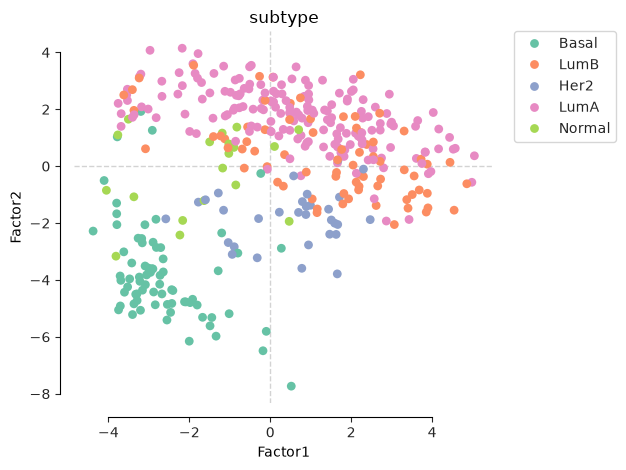
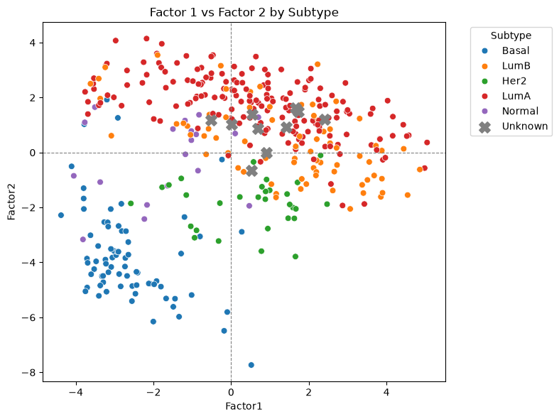
Visualise the factor space to see where the unknown samples fall relative to known subtypes
Classify each unknown sample as Luminal A / Luminal B using a simple logistic regression on the factors
Explain each prediction by finding the genes driving each unknown sample’s factor values, then linking those genes to diseases via a knowledge graph — to match against the clinical notes below
Answer — fill in your final
Pat_i -> TCGA-xxxxmapping
Patient clinical notes#
Prior to the accident, these are the disease/phenotype notes you recorded for each of the 10 patients whose samples are now mislabelled Pat_0 … Pat_9. You’ll use these — together with the molecular evidence gathered below — to work out which Pat_i is which TCGA-xxxx.
TCGA-EW-A6S9 — Presented with invasive breast carcinoma. Immunohistochemistry came back HER2-negative, but strongly positive for both estrogen and progesterone receptors, marking this out as a clearly hormone-receptor-driven tumor.
TCGA-A2-A0EP — Biopsy of a breast mass confirmed adenocarcinoma of ductal origin — glandular architecture arising from the mammary ducts, the most textbook presentation of the disease.
TCGA-E2-A1IG — A patient managing both asthma and Parkinson disease for several years, whose case took a sharp turn with the diagnosis of breast angiosarcoma, a rare and fast-growing vascular malignancy rather than a typical epithelial breast cancer.
TCGA-AQ-A1H3 — Decades of type 1 diabetes had already taken a toll by the time she came in: coronary artery disease and chronic kidney disease, the two classic downstream complications of long-standing diabetic vascular damage.
TCGA-AC-A2FE — Type 2 diabetes was already on the chart when breast angiosarcoma was diagnosed — a second, unrelated but noteworthy vascular malignancy layered onto an existing metabolic condition.
TCGA-A2-A1FX — Screening first picked up lobular neoplasia; further workup of a separate area of the breast then revealed medullary carcinoma, a less common but relatively well-differentiated histological subtype.
TCGA-A2-A4S3 — Living with multiple sclerosis, this patient went on to develop two independent primary cancers around the same time: an adenocarcinoma of the lung and a colorectal cancer, an unusually heavy cancer burden for one case.
TCGA-C8-A26W — Chronic kidney disease was a long-standing issue by the time gastric carcinoma appeared, and the picture was complicated further still by a later diagnosis of acute myeloid leukemia — three serious conditions converging in one patient.
TCGA-AR-A2LK — A palpable lump led to biopsy and a diagnosis of ductal adenocarcinoma of the breast, the same core histology as the most common form of breast adenocarcinoma.
TCGA-AO-A0JD — Type 2 diabetes was a pre-existing condition when this patient was diagnosed with breast angiosarcoma, a rare vascular tumor of the breast rather than the far more common ductal or lobular types.
1. Setup#
# Quick environment check (optional).
# Confirms the notebook is running on the expected machine / Python env / folder,
# since path or environment mismatches are a common source of confusing errors.
import socket
import os
import sys

print("Host:", socket.gethostname())
print("Python:", sys.executable)
print("Working dir:", os.getcwd())
Host: biomedicalai
Python: /opt/conda/envs/ECCB_2026/bin/python
Working dir: /home/bryan/ECCB2026_TEST/sessions/session-4-kg-query-mini-challenge
# ── Standard library ─────────────────────────────────────────────────────────
from pathlib import Path
import pickle

# ── Third-party ───────────────────────────────────────────────────────────────
import numpy as np
import pandas as pd
import matplotlib.pyplot as plt
import seaborn as sns
import networkx as nx
from matplotlib.colors import TwoSlopeNorm
from IPython.display import display

from sklearn.linear_model import LogisticRegression
# Extra metrics you may want once you've settled on a final answer and want to
# sanity-check a prediction against a partially-known label, or during model
# development on the labelled training cohort:
from sklearn.metrics import accuracy_score, balanced_accuracy_score, classification_report

# MOFA (Multi-Omics Factor Analysis): mofax is used to *read* a pretrained model.
# mofapy2 is only needed if you want to *train* a MOFA model from scratch, which
# isn't required for this challenge (a pretrained model is provided below).
import mofax as mfx

# ── Custom helpers for this workshop (see s4_helpers.py) ───────────────────────
from s4_helpers import (
    load_omics,
    evaluate_predictions,
    load_kg,
    print_graph_info,
    map_genes_to_kg,
    diseases_for_genes,
)

# ── Reproducibility ───────────────────────────────────────────────────────────
RANDOM_STATE = 42
2. Load data#
We need three things:
The 10 mislabelled “challenge” samples (
Pat_0…Pat_9) — these are the ones we’re re-identifying.The labelled training cohort used to train the MOFA model, plus the train/test patient ID split that was used at training time.
The pretrained MOFA model itself, so we can project the challenge samples into the same factor space.
# The 10 mislabelled samples for this challenge.
DATA_DIR = Path(".")

X_challenge_omics, y_challenge = load_omics(
    DATA_DIR,
    omic_filename="challenge_omics",
    omic_keys=["transcriptomics", "proteomics", "methylation"],
)

# The TCGA IDs Rocky mixed up (order not meaningful — this is what we're solving for).
missing_ids = [
    "TCGA-EW-A6S9", "TCGA-A2-A0EP", "TCGA-E2-A1IG",
    "TCGA-AQ-A1H3", "TCGA-AC-A2FE", "TCGA-A2-A1FX",
    "TCGA-A2-A4S3", "TCGA-C8-A26W", "TCGA-AR-A2LK", "TCGA-AO-A0JD",
]
pat_ids = [f"Pat_{i}" for i in range(10)]

# The true subtype of each challenge sample is unknown by construction — that's
# half of what we're inferring (the other half is the exact patient identity).
y_challenge["subtype"] = ["Unknown" for _ in range(10)]
y_challenge = y_challenge[["subtype"]]

# Relabel the challenge cohort with anonymised Pat_0..Pat_9 IDs.
for view in X_challenge_omics:
    X_challenge_omics[view].index = pat_ids
y_challenge.index = pat_ids

X_challenge_omics
Omic view dimensions:
  transcriptomics:   10 patients x  29995 features
  proteomics     :   10 patients x    464 features
  methylation    :   10 patients x 200000 features

Subtype counts:
subtype
Unknown    10
Name: count, dtype: int64
{'transcriptomics':        ENSG00000000003.15  ENSG00000000005.6  ENSG00000000419.13  \
 Pat_0           10.206609           3.890222           10.963447
 Pat_1           11.227947           7.885052           10.747011
 Pat_2           10.858597           3.622629           10.543180
 Pat_3           11.418415           6.649170           10.675950
 Pat_4           11.639118           7.683469           10.614152
 Pat_5           10.006381           3.991210           10.967056
 Pat_6           11.320906           4.597212           11.209474
 Pat_7           11.521549           4.382121           11.129100
 Pat_8           11.692278           4.079725           11.140742
 Pat_9           12.186842           4.716691           11.855058

        ENSG00000000457.14  ENSG00000000460.17  ENSG00000000938.13  \
 Pat_0            9.960213            8.783081            7.883629
 Pat_1           11.352407            8.963408           11.828274
 Pat_2           10.480666            8.805772            8.354700
 Pat_3           11.772228            9.739870            9.070792
 Pat_4           10.360072            8.960729            9.935186
 Pat_5            9.476851            8.826529            8.802416
 Pat_6           10.049028            9.896462            9.213614
 Pat_7           10.304102            9.837964            8.720828
 Pat_8           10.533073           10.023556            8.988475
 Pat_9           10.738790           10.903126            8.964495

        ENSG00000000971.16  ENSG00000001036.14  ENSG00000001084.13  \
 Pat_0           11.083770           10.744436           11.751679
 Pat_1           12.929817           11.243190           11.040297
 Pat_2           11.695405           10.179517           10.889103
 Pat_3           12.100870           10.894993            9.977176
 Pat_4           11.250770           11.529095           10.553126
 Pat_5           11.684284           11.000672           11.628035
 Pat_6           10.423992           12.156724           11.485138
 Pat_7           11.510676           12.033402           10.843561
 Pat_8           11.263677           10.980872           11.134081
 Pat_9            9.823592           13.432973           11.613547

        ENSG00000001167.14  ...  ENSG00000288611.1  ENSG00000288612.1  \
 Pat_0           11.388343  ...           4.450666           5.667865
 Pat_1           10.466207  ...           2.843467           6.377397
 Pat_2           11.436503  ...           4.163000           5.356899
 Pat_3           11.895307  ...           3.298848           5.391283
 Pat_4           11.372468  ...           2.843467           5.553009
 Pat_5           11.608577  ...           3.287055           6.508915
 Pat_6           11.997321  ...           5.576287           6.716968
 Pat_7           11.658691  ...           3.471029           6.382145
 Pat_8           11.812687  ...           3.518504           5.361268
 Pat_9           12.380097  ...           4.099344           4.571069

        ENSG00000288638.1  ENSG00000288648.1  ENSG00000288657.1  \
 Pat_0           2.843467           2.843467           3.375382
 Pat_1           2.843467           3.345657           2.843467
 Pat_2           2.843467           2.843467           3.397723
 Pat_3           2.843467           3.298848           2.843467
 Pat_4           2.843467           3.329320           2.843467
 Pat_5           2.843467           2.843467           2.843467
 Pat_6           2.843467           2.843467           2.843467
 Pat_7           2.843467           2.843467           3.471029
 Pat_8           2.843467           2.843467           2.843467
 Pat_9           2.843467           3.419187           2.843467

        ENSG00000288658.1  ENSG00000288663.1  ENSG00000288670.1  \
 Pat_0           3.591567           4.375290           8.897982
 Pat_1           5.122605           5.929506           7.922134
 Pat_2           3.622629           4.512358           9.500332
 Pat_3           3.625866           5.010104           8.810702
 Pat_4           4.768499           4.901473           8.606419
 Pat_5           3.468372           6.272242           8.215869
 Pat_6           4.937380           6.139969           8.373386
 Pat_7           3.724245           5.185608           8.314728
 Pat_8           3.666569           5.240143           9.601401
 Pat_9           3.828054           4.099344           7.871598

        ENSG00000288674.1  ENSG00000288675.1
 Pat_0           4.207402           5.903832
 Pat_1           4.776614           5.675877
 Pat_2           3.792194           5.234692
 Pat_3           4.234930           4.518756
 Pat_4           4.509409           5.603773
 Pat_5           4.201095           5.387085
 Pat_6           3.759852           4.860542
 Pat_7           3.824557           5.467033
 Pat_8           4.489482           4.489482
 Pat_9           3.419187           5.124520

 [10 rows x 29995 columns],
 'proteomics':        1433BETA  1433EPSILON  1433ZETA     4EBP1  4EBP1_pS65  4EBP1_pT37T46  \
 Pat_0  0.209990    -0.075390  0.371980 -0.224730   -0.485060      -0.692580
 Pat_1  0.312400     0.030429  0.253340 -0.611520   -0.201840       0.671530
 Pat_2  0.127790    -0.070532 -0.027055 -0.582010   -0.450870      -0.473950
 Pat_3  0.672860     0.454690  0.690000 -0.435830   -0.677050      -0.216300
 Pat_4  0.151560     0.191260  0.116100  0.007940   -0.475930       0.386940
 Pat_5 -0.145800     0.105943  0.923275  0.579005   -0.479165      -0.398805
 Pat_6  0.471200     0.135960  0.229710  0.421070   -0.820150      -0.588590
 Pat_7  0.266130     0.400270 -0.676650 -0.516900   -0.331410       0.146250
 Pat_8 -0.064925    -0.012983 -0.019147  0.122100   -0.503420       0.400560
 Pat_9  0.179010    -0.000011 -0.305770  0.387160   -0.403100      -0.892310

        4EBP1_pT70     53BP1  ACC_pS79      ACC1  ...       XPF     XRCC1  \
 Pat_0   -0.237400 -0.067915  0.081168  0.007453  ...  0.260623 -0.099892
 Pat_1   -0.490780 -0.814960  0.529520  0.870960  ...  0.298706 -0.115650
 Pat_2   -0.318360  0.360740  1.002400  0.899580  ...  0.620847  0.350880
 Pat_3   -0.325280 -1.454200  2.059000  0.801960  ...  0.635439 -0.797760
 Pat_4   -0.402460 -0.066013  0.806990  0.031855  ...  0.325157 -0.015553
 Pat_5   -0.006398 -0.010776  0.126345  0.721685  ... -0.006203 -0.149885
 Pat_6    0.402940 -0.669310 -0.067353 -0.189610  ...  0.559783  0.345610
 Pat_7    0.178840 -0.865140 -0.086904 -0.452800  ...  0.196953  0.150710
 Pat_8   -0.245610 -0.295440  0.246430  0.367050  ... -0.084701  0.126790
 Pat_9   -0.103780 -0.602700 -0.336820  0.341820  ... -0.226228 -0.024386

             YAP  YAP_pS127       YB1  YB1_pS102    YTHDF2    YTHDF3    ZAP-70  \
 Pat_0 -0.287960  -0.456050 -0.359370  -0.057382 -0.435499 -0.672054  0.516419
 Pat_1  0.049778   0.223490  0.037169   0.000000 -0.597347 -1.673852 -0.829929
 Pat_2 -0.272050  -0.422110  0.269720  -0.268640  0.450075 -0.159570 -0.370457
 Pat_3  1.320500   1.670100 -0.531290   0.322170 -1.465223 -0.971948 -0.591835
 Pat_4 -0.154470  -0.104590  0.326420  -0.141670 -0.160695  0.429300  1.105883
 Pat_5 -0.485700  -1.128265  0.203920  -0.249505  0.249155  0.477140 -0.294727
 Pat_6  0.249630  -0.449320 -0.368930   0.314880 -0.911570 -0.257785  1.340228
 Pat_7  0.373290   0.214090 -0.328940  -0.029406 -1.517599 -1.559424  0.885328
 Pat_8 -0.375900  -0.628490 -0.159960  -0.422880  0.027947  0.742192 -0.973856
 Pat_9 -0.339030  -0.793460 -0.252160   0.010017  0.671120  0.392285 -0.176342

            ZEB1
 Pat_0  0.364914
 Pat_1  0.282237
 Pat_2  0.434968
 Pat_3  0.912490
 Pat_4  0.431498
 Pat_5 -0.221702
 Pat_6  0.511333
 Pat_7  0.671174
 Pat_8  0.074150
 Pat_9 -0.122987

 [10 rows x 464 columns],
 'methylation':        cg11738485  cg01893212  cg23179456  cg12466610  cg22473620  cg15690342  \
 Pat_0    0.036465    0.459944    0.765009    0.523401    0.666596    0.171290
 Pat_1    0.642683    0.366179    0.147451    0.082516    0.234550    0.329291
 Pat_2    0.587153    0.808454    0.802197    0.598610    0.793824    0.825494
 Pat_3    0.559811    0.694687    0.661540    0.230455    0.499805    0.755860
 Pat_4    0.984174    0.585158    0.581683    0.290122    0.598232    0.629066
 Pat_5    0.015636    0.750984    0.780966    0.469563    0.737902    0.572635
 Pat_6    0.029568    0.030172    0.660712    0.548529    0.721839    0.184347
 Pat_7    0.727794    0.039441    0.030866    0.971210    0.345076    0.237567
 Pat_8    0.981246    0.829965    0.660667    0.055368    0.041200    0.849246
 Pat_9    0.680905    0.046090    0.837534    0.614237    0.798068    0.886255

        cg02467990  cg21885317  cg20399616  cg22831607  ...  cg03082813  \
 Pat_0    0.309456    0.087059    0.146893    0.304569  ...    0.099009
 Pat_1    0.343183    0.929976    0.146072    0.168229  ...    0.111423
 Pat_2    0.767110    0.951831    0.768201    0.042451  ...    0.047717
 Pat_3    0.643704    0.192525    0.652058    0.669029  ...    0.072981
 Pat_4    0.509020    0.905908    0.616243    0.629752  ...    0.086513
 Pat_5    0.714676    0.330090    0.758003    0.295251  ...    0.084584
 Pat_6    0.021985    0.937415    0.039530    0.585501  ...    0.088012
 Pat_7    0.040871    0.170520    0.099211    0.062540  ...    0.048544
 Pat_8    0.812736    0.695391    0.802597    0.868684  ...    0.097715
 Pat_9    0.041928    0.931980    0.742047    0.672269  ...    0.047196

        cg13744910  cg09550558  cg09395540  cg13222853  cg06575013  cg23123972  \
 Pat_0    0.964663    0.122532    0.922226    0.869302    0.093457    0.851539
 Pat_1    0.972984    0.069577    0.948352    0.883429    0.126899    0.910045
 Pat_2    0.965976    0.064062    0.821157    0.910605    0.078588    0.926255
 Pat_3    0.973397    0.070123    0.937828    0.911747    0.095471    0.893391
 Pat_4    0.971771    0.066935    0.938623    0.896895    0.114243    0.882909
 Pat_5    0.964760    0.064851    0.873053    0.930288    0.093407    0.912283
 Pat_6    0.958149    0.087123    0.917065    0.863395    0.097908    0.848616
 Pat_7    0.975608    0.079897    0.934193    0.871475    0.149388    0.933717
 Pat_8    0.976676    0.079897    0.829877    0.882533    0.105870    0.885309
 Pat_9    0.976905    0.071415    0.904568    0.928623    0.080946    0.671952

        cg10507099  cg03538345  cg14015726
 Pat_0    0.019959    0.166893    0.941172
 Pat_1    0.017771    0.127076    0.944468
 Pat_2    0.017049    0.111346    0.953182
 Pat_3    0.018662    0.104881    0.918535
 Pat_4    0.016234    0.087803    0.947652
 Pat_5    0.020630    0.069685    0.933060
 Pat_6    0.021112    0.094935    0.812604
 Pat_7    0.022462    0.163373    0.943986
 Pat_8    0.017831    0.147168    0.934284
 Pat_9    0.016314    0.088723    0.943192

 [10 rows x 200000 columns]}
# The labelled training cohort (TCGA-BRCA) that the MOFA model below was trained on.
TRAIN_DATA_DIR = Path("/data/")

X_omics, y = load_omics(
    TRAIN_DATA_DIR,
    omic_filename="omics",
    omic_keys=["transcriptomics", "proteomics", "methylation"],
)

with open(TRAIN_DATA_DIR / "patient_splits.pkl", "rb") as f:
    splits = pickle.load(f)

train_ids = splits["train_ids"]
test_ids = splits["test_ids"]

# Split the labels using the same patient IDs used for the omics data.
y_train = y.loc[train_ids]
y_test = y.loc[test_ids]
Omic view dimensions:
  transcriptomics:  500 patients x  29995 features
  proteomics     :  500 patients x    464 features
  methylation    :  500 patients x 200000 features

Subtype counts:
paper_BRCA_Subtype_PAM50
LumA      237
LumB      100
Basal      97
Her2       41
Normal     25
Name: count, dtype: int64
# Load the pretrained MOFA model.
mofa_model_mfx = mfx.mofa_model("mofa_pretrained.hdf5")

print(mofa_model_mfx)          # Model overview
print(mofa_model_mfx.shape)    # (n_samples, n_factors)

# Extract key components.
factors = mofa_model_mfx.get_factors(df=True)               # Factor/latent space values
weights = mofa_model_mfx.get_weights(df=True)         # Feature weights/loadings
var_exp = mofa_model_mfx.get_variance_explained()     # R^2 per factor per view

# NOTE: the exact factor-name format (e.g. "Factor1" vs "Factor 1") depends on
# your mofax version. Check this before relying on either format later in the
# notebook:
print("Factor column names look like:", list(factors.columns[:3]))
MOFA+ model: mofa pretrained
Samples (cells): 375
Features: 4464
Groups: TCGA-BRCA_train (375)
Views: methylation (2000), proteomics (464), transcriptomics (2000)
Factors: 10
Expectations: W, Z
(375, 4464)
Factor column names look like: ['Factor1', 'Factor2', 'Factor3']
3. Project the challenge samples into the MOFA factor space#
MOFA was fit on the training cohort only. To place the 10 unknown challenge samples on the same latent axes, we need to project them using the feature weights the model already learned — without ever touching the (unknown) labels.
# Restrict each omics view to the features MOFA actually used (its most-variable,
# training-selected feature set), so train and test matrices line up column-for-column.
X_train_raw = {name: X.loc[train_ids] for name, X in X_omics.items()}
X_test_raw = {name: X for name, X in X_challenge_omics.items()}

features_in_mofa = set(weights.index)
X_train_omics = {}
X_test_omics = {}

for name, X_train_view in X_train_raw.items():
    selected_features = list(features_in_mofa & set(X_train_view.columns))
    X_train_omics[name] = X_train_view.loc[:, selected_features]
    X_test_omics[name] = X_test_raw[name].loc[:, selected_features]

print("Feature counts after filtering to MOFA's feature set:")
for name in X_omics:
    print(
        f"  {name:15s}: {X_omics[name].shape[1]:6d} original -> "
        f"{X_train_omics[name].shape[1]:6d} used by MOFA"
    )
Feature counts after filtering to MOFA's feature set:
  transcriptomics:  29995 original ->   2000 used by MOFA
  proteomics     :    464 original ->    464 used by MOFA
  methylation    : 200000 original ->   2000 used by MOFA
def project_test_patients_to_mofa_factors(model, X_train_by_view, X_test_by_view, train_factors, view_names):
    """Project held-out patients into the fixed MOFA factor space.

    The projection uses MOFA weights learned from training patients. To keep
    train and test factor values comparable, preprocessing and calibration are
    fit on training patients only and then applied unchanged to test patients
    (test labels are never used anywhere in this function).
    """
    factor_columns = train_factors.columns.astype(str).tolist()
    projected_test_by_view = []

    for view_name in view_names:
        # W is the learned feature x factor weight matrix for this omics view.
        view_weights = model.get_weights(views=view_name, df=True)
        view_weights.columns = view_weights.columns.astype(str)
        view_weights = view_weights.reindex(columns=factor_columns)

        # Use only features present in the trained weights AND both train/test matrices.
        common_features = view_weights.index.intersection(X_train_by_view[view_name].columns)
        common_features = common_features.intersection(X_test_by_view[view_name].columns)
        view_weights = view_weights.loc[common_features]

        X_train_view = X_train_by_view[view_name].loc[:, common_features].astype(float)
        X_test_view = X_test_by_view[view_name].loc[:, common_features].astype(float)
        X_train_view.index = X_train_view.index.astype(str)
        X_test_view.index = X_test_view.index.astype(str)

        # Learn centering/scaling on training patients only, then apply it to test patients.
        train_mean = X_train_view.mean(axis=0)
        train_std = X_train_view.std(axis=0, ddof=0).replace(0, 1)
        X_train_scaled = (X_train_view - train_mean) / train_std
        X_test_scaled = (X_test_view - train_mean) / train_std

        # Project X into the fixed MOFA weight space via the pseudo-inverse of W.
        raw_train_projection = X_train_scaled.to_numpy() @ np.linalg.pinv(view_weights.to_numpy()).T
        raw_test_projection = X_test_scaled.to_numpy() @ np.linalg.pinv(view_weights.to_numpy()).T

        # Calibrate the raw projection to the factor scale returned by the trained
        # MOFA model. Fitted on training patients only; test labels are never used.
        train_design = np.column_stack([raw_train_projection, np.ones(raw_train_projection.shape[0])])
        test_design = np.column_stack([raw_test_projection, np.ones(raw_test_projection.shape[0])])
        train_target = train_factors.loc[X_train_view.index, factor_columns].to_numpy()
        calibration = np.linalg.lstsq(train_design, train_target, rcond=None)[0]
        projected_values = test_design @ calibration

        projected = pd.DataFrame(projected_values, index=X_test_view.index, columns=factor_columns)
        projected_test_by_view.append(projected)

    # Each view gives one projected factor table; average them since all views
    # are available for every challenge sample here.
    return sum(projected_test_by_view) / len(projected_test_by_view)
# Extract training-patient factor values straight from the fitted MOFA model.
train_factors_mfx = mofa_model_mfx.get_factors(df=True)
train_factors_mfx.index = train_factors_mfx.index.astype(str)

# Project the 10 held-out challenge patients into that same factor space.
test_factors_mfx = project_test_patients_to_mofa_factors(
    mofa_model_mfx,
    X_train_omics,
    X_test_omics,
    train_factors_mfx,
    list(X_train_omics.keys()),
)
# Attach the known training subtypes to the model so mofax's built-in plots can
# colour training points by subtype.
mofa_sample_metadata = pd.DataFrame(index=train_factors_mfx.index)
mofa_sample_metadata["subtype"] = y_train.reindex(train_factors_mfx.index).values

mofa_model_mfx.samples_metadata = mofa_sample_metadata
4. Visualise the factor space#
# Built-in mofax scatter grid, training patients only, coloured by subtype.
mfx.plot_factors_scatter(
    mofa_model_mfx,
    x="Factor1",
    y="Factor2",
    group_label="subtype",
    color="subtype",
    zero_line_x=True,
    zero_line_y=True,
    ncols=3,
    size=40,
    alpha=1,
)
plt.show()
# Combine training (known subtype) and challenge (unknown subtype) factors into
# one long table we can reuse for every plot below.
plot_df = pd.concat([train_factors_mfx, test_factors_mfx])

subtypes_col = pd.concat([
    y_train,
    pd.Series(["Unknown"] * len(test_factors_mfx), index=test_factors_mfx.index),
])
plot_df["subtype"] = subtypes_col

plot_df
| Factor1 | Factor2 | Factor3 | Factor4 | Factor5 | Factor6 | Factor7 | Factor8 | Factor9 | Factor10 | subtype | |
|---|---|---|---|---|---|---|---|---|---|---|---|
| TCGA-S3-AA0Z | -2.677049 | -4.491632 | 1.438483 | -0.422795 | 0.741272 | 1.235917 | 1.497584 | -0.306961 | 0.952876 | -0.117106 | Basal |
| TCGA-E9-A1N6 | 0.180977 | -0.561914 | -3.574715 | -2.498562 | -3.337365 | -2.594017 | -1.536899 | 1.478458 | -0.399653 | 1.112885 | LumB |
| TCGA-C8-A26Y | -1.037958 | -2.685832 | 0.221065 | -2.129348 | -1.283929 | -3.698094 | -2.550864 | 3.238068 | 0.323258 | 0.714914 | Her2 |
| TCGA-A7-A0D9 | 0.757382 | -0.338205 | -1.839327 | 6.520308 | -4.192802 | 1.799493 | -0.594609 | 1.617057 | -4.788059 | 2.172852 | LumA |
| TCGA-A2-A0CT | 4.982207 | -0.566879 | 0.930730 | -0.789196 | -1.455145 | 2.251426 | 3.763444 | 1.592921 | 0.738021 | 0.874641 | LumA |
| ... | ... | ... | ... | ... | ... | ... | ... | ... | ... | ... | ... |
| Pat_5 | 1.732713 | 1.484934 | 0.798178 | -0.922396 | -0.938942 | 2.177108 | -1.136659 | 0.900399 | -0.561686 | -0.393969 | Unknown |
| Pat_6 | 0.525045 | -0.649719 | 0.079504 | -1.348195 | 1.465892 | 0.453576 | -1.885745 | 0.881061 | -0.181360 | 0.944625 | Unknown |
| Pat_7 | -0.511048 | 1.179021 | -1.281183 | -0.298532 | 0.825806 | -0.048020 | -1.702661 | -0.368831 | 0.132252 | 0.810454 | Unknown |
| Pat_8 | 2.410831 | 1.197439 | 1.041670 | -1.269500 | -0.668765 | 0.721102 | 0.172933 | -1.027378 | -0.076351 | 0.376981 | Unknown |
| Pat_9 | 0.916728 | 0.003875 | 0.923834 | -0.510366 | 0.090924 | -0.598543 | -1.956078 | 0.735629 | 0.040657 | -0.187265 | Unknown |
385 rows × 11 columns
fig, ax = plt.subplots(figsize=(8, 6))

# Split known vs unknown subtypes (handles both NaN and the literal 'Unknown' label).
known = plot_df[plot_df["subtype"].notna() & ~plot_df["subtype"].isin(["Unknown"])]
unknown = plot_df[plot_df["subtype"].isna() | plot_df["subtype"].isin(["Unknown"])]

# Known subtypes as coloured circles.
sns.scatterplot(data=known, x="Factor1", y="Factor2", hue="subtype", s=40, alpha=1, ax=ax)

# Unknown (challenge) samples as bigger grey crosses, drawn on top.
ax.scatter(
    unknown["Factor1"], unknown["Factor2"],
    marker="X", s=120, color="grey", label="Unknown", zorder=5, linewidths=1.2,
)

ax.axhline(0, color="grey", linewidth=0.8, linestyle="--")
ax.axvline(0, color="grey", linewidth=0.8, linestyle="--")
ax.set_title("Factor 1 vs Factor 2 by Subtype")
ax.legend(title="Subtype", bbox_to_anchor=(1.05, 1), loc="upper left")
plt.tight_layout()
plt.show()
4.1 Compare subtypes across a wider set of factors#
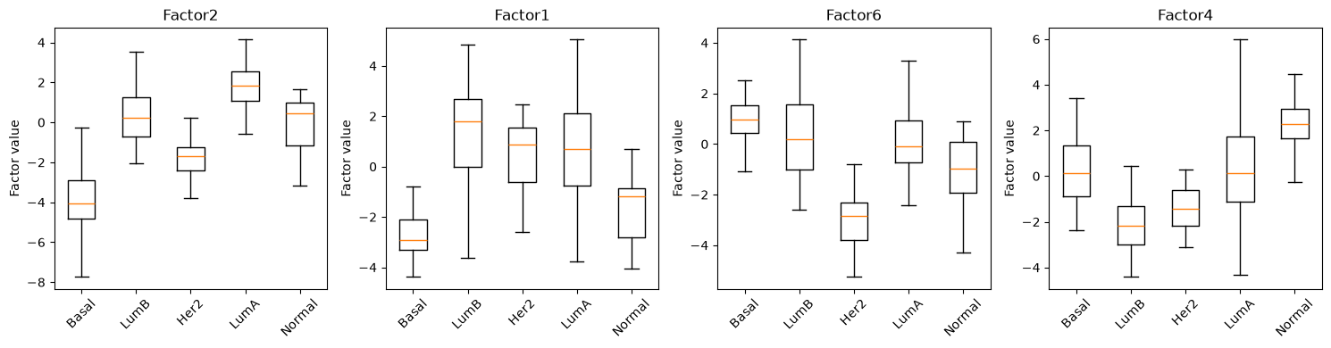
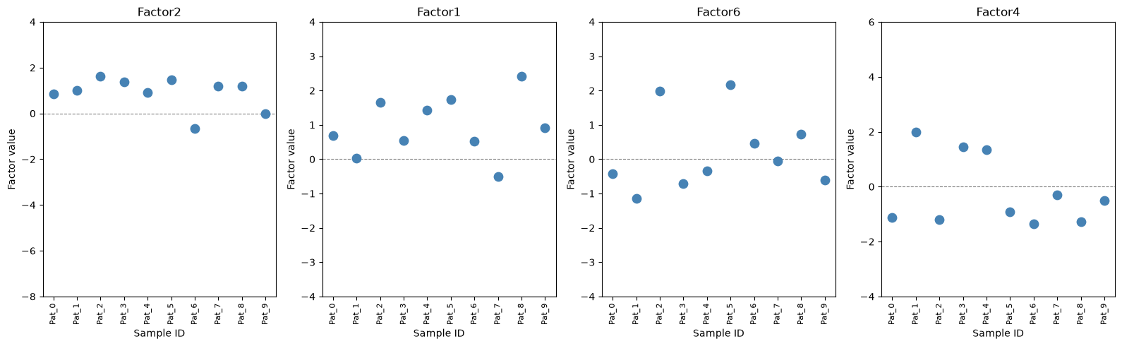
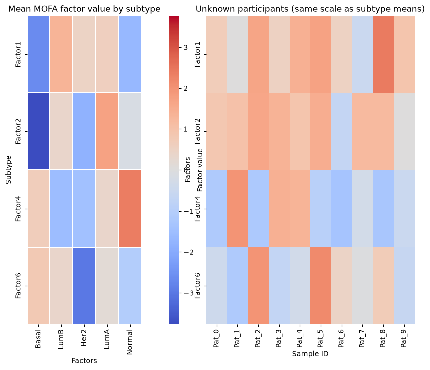
Two factors aren’t always enough to separate every subtype — below we look at a few more factors as boxplots (by known subtype) and then as individual scatter points for the unknown samples, so we can eyeball which subtype each challenge sample is likely to belong to before formally classifying it in Section 5.
subtype_order = ["Basal", "LumB", "Her2", "LumA", "Normal"]
factors_of_interest = ["Factor2", "Factor1", "Factor6", "Factor4"]

fig, axes = plt.subplots(1, len(factors_of_interest), figsize=(15, 4), squeeze=False)

for ax, factor in zip(axes.ravel(), factors_of_interest):
    groups = [
        plot_df.loc[plot_df["subtype"] == subtype, factor].dropna()
        for subtype in subtype_order
    ]
    ax.boxplot(groups, tick_labels=subtype_order, showfliers=False)
    ax.set_title(factor)
    ax.set_ylabel("Factor value")
    ax.tick_params(axis="x", rotation=45)

plt.tight_layout()
plt.show()
# Y-axis limits per factor, just for a bit of visual polish.
ylims = {
    "Factor2": (-8, 4),
    "Factor1": (-4, 4),
    "Factor6": (-4, 4),
    "Factor4": (-4, 6),
}

unknown_df = plot_df[plot_df["subtype"] == "Unknown"]

fig, axes = plt.subplots(1, len(factors_of_interest), figsize=(16, 5), squeeze=False)

for ax, factor in zip(axes.ravel(), factors_of_interest):
    vals = unknown_df[factor].dropna()

    ax.scatter(range(len(vals)), vals.values, s=80, color="steelblue", zorder=5)
    ax.set_xticks(range(len(vals)))
    ax.set_xticklabels(vals.index, rotation=90, fontsize=8)
    ax.axhline(0, color="grey", linewidth=0.8, linestyle="--")
    ax.set_ylim(ylims[factor])
    ax.set_title(factor)
    ax.set_ylabel("Factor value")
    ax.set_xlabel("Sample ID")

plt.tight_layout()
plt.show()
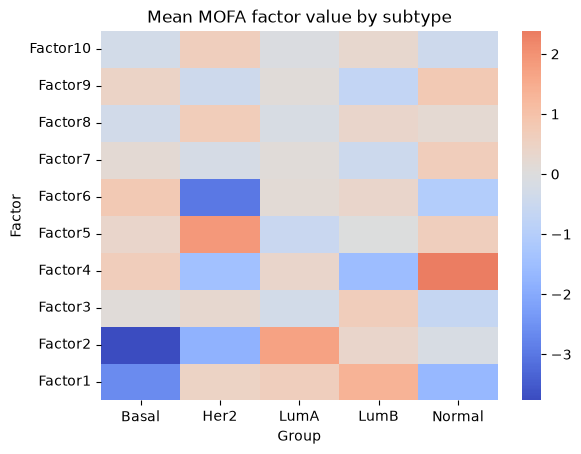
# Built-in mofax heatmap of the mean factor value per subtype (training patients only —
# challenge patients have subtype == NaN/'Unknown' so they don't contribute here).
mfx.plot_factors_matrix(
    mofa_model_mfx,
    group_label="subtype",
    cmap="coolwarm",
    center=0,
)
plt.title("Mean MOFA factor value by subtype")
plt.show()
# Recreate that same subtype-mean heatmap side-by-side with the unknown samples,
# on a shared colour scale, so it's easy to visually match each unknown sample's
# row-pattern to the subtype it most resembles.
heatmap_factors = [f"Factor{i}" for i in [1, 2, 4, 6]]

unknown_mask = plot_df["subtype"].isna() | plot_df["subtype"].isin(["Unknown", "NA", "unknown"])

unknown_mat = plot_df.loc[unknown_mask, heatmap_factors].dropna(how="all")
heat_unknown = unknown_mat.T  # rows = factors, cols = sample IDs

means_by_subtype = (
    plot_df.loc[~unknown_mask, ["subtype"] + heatmap_factors]
    .dropna(subset=["subtype"])
    .groupby("subtype")[heatmap_factors]
    .mean()
    .reindex(subtype_order)
)

# Colour scale is defined ONLY from the subtype-mean matrix, so the unknown
# heatmap is shown on the exact same scale as the reference panel.
vmax = np.nanmax(np.abs(means_by_subtype.values))
norm = TwoSlopeNorm(vmin=-vmax, vcenter=0.0, vmax=vmax)

fig = plt.figure(figsize=(max(10, 0.35 * heat_unknown.shape[1] + 6), 8))
gs = fig.add_gridspec(1, 3, width_ratios=[2.2, 0.18, max(4, 0.35 * heat_unknown.shape[1])], wspace=0.25)

ax_ref = fig.add_subplot(gs[0, 0])
cax = fig.add_subplot(gs[0, 1])
ax_unk = fig.add_subplot(gs[0, 2])

sns.heatmap(means_by_subtype.T, ax=ax_ref, cmap="coolwarm", norm=norm, cbar=False,
            linewidths=0.2, linecolor="white")
ax_ref.set_title("Mean MOFA factor value by subtype")
ax_ref.set_xlabel("Factors")
ax_ref.set_ylabel("Subtype")
ax_ref.tick_params(axis="x", rotation=90)

sns.heatmap(heat_unknown, ax=ax_unk, cmap="coolwarm", norm=norm, cbar=True,
            cbar_ax=cax, linewidths=0.0)
ax_unk.set_title("Unknown participants (same scale as subtype means)")
ax_unk.set_xlabel("Sample ID")
ax_unk.set_ylabel("Factors")
ax_unk.tick_params(axis="x", rotation=90)

cax.set_ylabel("Factor value")
plt.tight_layout()
plt.show()
/tmp/ipykernel_1508621/1113544594.py:46: UserWarning: This figure includes Axes that are not compatible with tight_layout, so results might be incorrect.
  plt.tight_layout()
5. Classify each unknown sample: Luminal A or Luminal B#
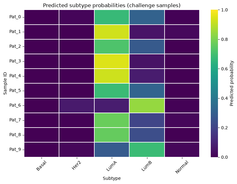
We already know (from earlier statistics) that all 10 unknown samples are either Luminal A or Luminal B. A simple logistic regression on the MOFA factors — trained on the labelled cohort — gives us a first, quantitative pass at this split, which we can combine with the visual read from Section 4.
# 1) Get y_train as a 1D Series of subtype labels.
subtype_labels = y_train
if isinstance(subtype_labels, pd.DataFrame):
    if "paper_BRCA_Subtype_PAM50" in subtype_labels.columns:
        subtype_labels = subtype_labels["paper_BRCA_Subtype_PAM50"]
    elif "subtype" in subtype_labels.columns:
        subtype_labels = subtype_labels["subtype"]
    else:
        raise ValueError("Could not find a subtype column in y_train.")

# 2) Align train X and y by sample IDs.
common_ids = train_factors_mfx.index.intersection(subtype_labels.index)
X_train_clf = train_factors_mfx.loc[common_ids]
y_train_clf = subtype_labels.loc[common_ids]

# 3) Fit a simple multi-class logistic regression on all factors.
clf = LogisticRegression(solver="lbfgs", max_iter=5000, random_state=RANDOM_STATE)
clf.fit(X_train_clf, y_train_clf)

# 4) Predict on the challenge (unknown) samples.
test_pred = clf.predict(test_factors_mfx)
predicted_subtype = pd.Series(test_pred, index=test_factors_mfx.index, name="predicted_subtype")

predicted_subtype
Pat_0    LumA
Pat_1    LumA
Pat_2    LumA
Pat_3    LumA
Pat_4    LumA
Pat_5    LumA
Pat_6    LumB
Pat_7    LumA
Pat_8    LumA
Pat_9    LumB
Name: predicted_subtype, dtype: str
predicted_proba = pd.DataFrame(
    clf.predict_proba(test_factors_mfx),
    index=test_factors_mfx.index,
    columns=clf.classes_,
)

fig, ax = plt.subplots(figsize=(8, max(6, 0.25 * predicted_proba.shape[0])))

sns.heatmap(
    predicted_proba,
    cmap="viridis",
    vmin=0, vmax=1,
    linewidths=0.2,
    linecolor="white",
    cbar_kws={"label": "Predicted probability"},
    ax=ax,
)
ax.set_title("Predicted subtype probabilities (challenge samples)")
ax.set_xlabel("Subtype")
ax.set_ylabel("Sample ID")
ax.tick_params(axis="x", rotation=45)
ax.tick_params(axis="y", rotation=0)

plt.tight_layout()
plt.show()

predicted_proba
| Basal | Her2 | LumA | LumB | Normal | |
|---|---|---|---|---|---|
| Pat_0 | 3.847440e-05 | 0.013562 | 0.671983 | 0.310265 | 0.004151 |
| Pat_1 | 2.466155e-04 | 0.000998 | 0.926213 | 0.051993 | 0.020549 |
| Pat_2 | 2.847282e-07 | 0.000012 | 0.719408 | 0.280566 | 0.000013 |
| Pat_3 | 2.101006e-05 | 0.000099 | 0.947450 | 0.049191 | 0.003239 |
| Pat_4 | 1.386258e-05 | 0.000172 | 0.923490 | 0.074452 | 0.001872 |
| Pat_5 | 4.128784e-07 | 0.000006 | 0.683015 | 0.316967 | 0.000012 |
| Pat_6 | 2.432563e-03 | 0.068885 | 0.081754 | 0.841215 | 0.005713 |
| Pat_7 | 3.578692e-04 | 0.004467 | 0.770673 | 0.206939 | 0.017563 |
| Pat_8 | 4.269855e-07 | 0.000212 | 0.761841 | 0.237774 | 0.000172 |
| Pat_9 | 1.166027e-03 | 0.016971 | 0.281572 | 0.682959 | 0.017332 |
6. Explain each unknown sample: driving genes -> diseases#
Knowing Luminal A vs B narrows things down but doesn’t tell us which patient a sample belongs to. For that we look at which genes most strongly drive each unknown sample’s position in factor space, then look up which diseases those genes are associated with in a knowledge graph — so we can match against the clinical notes at the top of the notebook.
We run this for all 10 unknown samples (not just one), since we need to
resolve every Pat_i.
def top_features_weighted_by_expression(
    model,
    X: pd.DataFrame,
    sample_id: str,
    factor: str,
    view: str,
    top_n: int = 20,
    standardize: bool = True,
):
    """Rank features for one sample/factor by |weight| * |expression|.

    A feature's contribution to a sample's factor value is roughly proportional
    to its MOFA weight times how far that sample's (standardized) expression is
    from the cohort mean. Sorting by this product surfaces the genes that most
    plausibly explain *why* this particular sample sits where it does on this factor.
    """
    # W: features x factors
    W = model.get_weights(views=view, df=True)
    w = W[factor]

    x = X.loc[sample_id]
    if standardize:
        # z-score each feature across samples so weight and expression are comparable.
        x = (x - X.mean(axis=0)) / X.std(axis=0).replace(0, pd.NA)

    impact = (w.abs() * x.abs()).dropna().sort_values(ascending=False)

    out = pd.DataFrame({
        "weight_abs": w.abs().reindex(impact.index),
        "x_abs": x.abs().reindex(impact.index),
        "impact": impact,
    })
    return out.head(top_n)
# Which factors and view to explain each sample with. Factor1/2/4/6 were the
# ones that visually separated subtypes best in Section 4 — feel free to widen
# this set (or try 'proteomics'/'methylation') if your matches aren't conclusive.
factors_to_explain = ["Factor1", "Factor2", "Factor4", "Factor6"]
view = "transcriptomics"

# top_genes_by_sample: {sample_id -> list of top driving gene names}
top_genes_by_sample = {}

for sample_id in unknown_df.index:
    genes_for_this_sample = []
    for factor in factors_to_explain:
        top = top_features_weighted_by_expression(
            mofa_model_mfx,
            X_test_omics[view],
            sample_id=sample_id,
            factor=factor,
            view=view,
            top_n=25,
        )
        genes_for_this_sample += list(top.index)
    top_genes_by_sample[sample_id] = sorted(set(genes_for_this_sample))

for sample_id, genes in top_genes_by_sample.items():
    print(f"{sample_id}: {len(genes)} candidate driving genes")
Pat_0: 84 candidate driving genes
Pat_1: 89 candidate driving genes
Pat_2: 85 candidate driving genes
Pat_3: 91 candidate driving genes
Pat_4: 82 candidate driving genes
Pat_5: 85 candidate driving genes
Pat_6: 83 candidate driving genes
Pat_7: 78 candidate driving genes
Pat_8: 85 candidate driving genes
Pat_9: 83 candidate driving genes
# Load the gene-disease knowledge graph once.
G = load_kg()
print_graph_info(G)
Number of nodes: 881
Number of edges: 1768
Graph type: undirected

Nodes by type:
     760  gene
      90  disease
      31  icd10
Edges by type:
   1,656  associated_with
      81  is_a
      31  maps_to

Self-loops: 0
Graph density: 0.004561
Connected components: 1
Largest component: 881 nodes (100.0% of the graph)
Average clustering coefficient: 0.0137
# For each unknown sample, map its driving genes onto the KG and pull the
# diseases most associated with them — these are the clues to match against
# the clinical notes at the top of the notebook.
disease_hits_by_sample = {}

for sample_id, genes in top_genes_by_sample.items():
    mapped = map_genes_to_kg(G, genes)
    n_in_kg = mapped["in_kg"].sum()

    diseases = diseases_for_genes(G, genes, top_n=30)
    disease_hits_by_sample[sample_id] = diseases

    print(f"\n=== {sample_id}: {n_in_kg} / {len(mapped)} genes found in KG ===")
    display(diseases.head(10))
=== Pat_0: 8 / 84 genes found in KG ===
| disease_id | name | n_genes | mean_score | genes | |
|---|---|---|---|---|---|
| 0 | MONDO_0006512 | estrogen-receptor positive breast cancer | 4 | 0.342725 | ARHGEF38, CCDC170, ESR1, NEK10 |
| 1 | MONDO_0000618 | Her2-receptor negative breast cancer | 4 | 0.237250 | CCDC170, DNER, ESR1, NEK10 |
| 2 | MONDO_0006513 | estrogen-receptor negative breast cancer | 3 | 0.305100 | CCDC170, ESR1, NEK10 |
| 3 | MONDO_0007254 | breast cancer | 2 | 0.681400 | ERBB2, ESR1 |
| 4 | MONDO_0004950 | gastric carcinoma | 2 | 0.432450 | ERBB2, ESR1 |
| 5 | MONDO_0004989 | breast carcinoma | 2 | 0.704800 | ERBB2, ESR1 |
| 6 | MONDO_0006244 | HER2 positive breast carcinoma | 2 | 0.541300 | ERBB2, ESR1 |
| 7 | MONDO_0021115 | luminal B breast carcinoma | 2 | 0.373450 | CCDC170, ESR1 |
| 8 | MONDO_0004988 | breast adenocarcinoma | 2 | 0.581300 | ERBB2, ESR1 |
| 9 | MONDO_0005298 | osteoporosis | 2 | 0.567900 | CCDC170, ESR1 |
=== Pat_1: 8 / 89 genes found in KG ===
| disease_id | name | n_genes | mean_score | genes | |
|---|---|---|---|---|---|
| 0 | MONDO_0021115 | luminal B breast carcinoma | 3 | 0.331667 | ESR1, FOXA1, GATA3 |
| 1 | MONDO_0004988 | breast adenocarcinoma | 3 | 0.548900 | ESR1, FOXA1, GATA3 |
| 2 | MONDO_0006116 | breast carcinoma by gene expression profile | 3 | 0.370000 | ESR1, FOXA1, GATA3 |
| 3 | MONDO_0005590 | breast ductal adenocarcinoma | 3 | 0.379933 | ESR1, FOXA1, GATA3 |
| 4 | MONDO_0005298 | osteoporosis | 2 | 0.577850 | ESR1, PGR |
| 5 | MONDO_0000552 | breast lobular carcinoma | 2 | 0.379500 | ESR1, FOXA1 |
| 6 | EFO_0009782 | progesterone-receptor positive breast cancer | 2 | 0.178700 | ESR1, THSD4 |
| 7 | MONDO_0005063 | medullary breast carcinoma | 2 | 0.139350 | ESR1, MUC16 |
| 8 | MONDO_0004379 | female breast carcinoma | 2 | 0.324100 | ESR1, GATA3 |
| 9 | MONDO_0000618 | Her2-receptor negative breast cancer | 2 | 0.313500 | ESR1, THSD4 |
=== Pat_2: 4 / 85 genes found in KG ===
| disease_id | name | n_genes | mean_score | genes | |
|---|---|---|---|---|---|
| 0 | MONDO_0003024 | breast angiosarcoma | 2 | 0.08565 | ADIPOQ, IL33 |
| 1 | MONDO_0004979 | asthma | 1 | 0.71850 | IL33 |
| 2 | MONDO_0008315 | prostate cancer | 1 | 0.79930 | AR |
| 3 | MONDO_0005298 | osteoporosis | 1 | 0.48990 | AR |
| 4 | MONDO_0005590 | breast ductal adenocarcinoma | 1 | 0.37290 | AR |
| 5 | MONDO_0006244 | HER2 positive breast carcinoma | 1 | 0.37000 | AR |
| 6 | MONDO_0006043 | metaplastic breast carcinoma | 1 | 0.27840 | AR |
| 7 | MONDO_0004379 | female breast carcinoma | 1 | 0.27810 | AR |
| 8 | EFO_0009782 | progesterone-receptor positive breast cancer | 1 | 0.07400 | AR |
| 9 | MONDO_0005180 | Parkinson disease | 1 | 0.61020 | MAPT |
=== Pat_3: 11 / 91 genes found in KG ===
| disease_id | name | n_genes | mean_score | genes | |
|---|---|---|---|---|---|
| 0 | MONDO_0006512 | estrogen-receptor positive breast cancer | 2 | 0.3263 | ARHGEF38, NEK10 |
| 1 | MONDO_0006513 | estrogen-receptor negative breast cancer | 2 | 0.2624 | LGR6, NEK10 |
| 2 | MONDO_0021115 | luminal B breast carcinoma | 2 | 0.2775 | ERBB4, GATA3 |
| 3 | MONDO_0004988 | breast adenocarcinoma | 1 | 0.5676 | GATA3 |
| 4 | MONDO_0005298 | osteoporosis | 1 | 0.4447 | PGR |
| 5 | MONDO_0005147 | type 1 diabetes mellitus | 1 | 0.5100 | SLC5A1 |
| 6 | MONDO_0005300 | chronic kidney disease | 1 | 0.4716 | SLC5A1 |
| 7 | MONDO_0004379 | female breast carcinoma | 1 | 0.3700 | GATA3 |
| 8 | MONDO_0005590 | breast ductal adenocarcinoma | 1 | 0.3731 | GATA3 |
| 9 | MONDO_0006256 | invasive breast carcinoma | 1 | 0.3772 | GATA3 |
=== Pat_4: 4 / 82 genes found in KG ===
| disease_id | name | n_genes | mean_score | genes | |
|---|---|---|---|---|---|
| 0 | MONDO_0005148 | type 2 diabetes mellitus | 1 | 0.8566 | ABCC8 |
| 1 | MONDO_0006513 | estrogen-receptor negative breast cancer | 1 | 0.2838 | OSR1 |
| 2 | MONDO_0000552 | breast lobular carcinoma | 1 | 0.3700 | AFF3 |
| 3 | MONDO_0006116 | breast carcinoma by gene expression profile | 1 | 0.2775 | AFF3 |
| 4 | MONDO_0003024 | breast angiosarcoma | 1 | 0.0681 | ADIPOQ |
=== Pat_5: 4 / 85 genes found in KG ===
| disease_id | name | n_genes | mean_score | genes | |
|---|---|---|---|---|---|
| 0 | MONDO_0002486 | lobular neoplasia | 1 | 0.0812 | CD36 |
| 1 | MONDO_0003024 | breast angiosarcoma | 1 | 0.0681 | ADIPOQ |
| 2 | MONDO_0005063 | medullary breast carcinoma | 1 | 0.0925 | MUC16 |
| 3 | MONDO_0006117 | breast diffuse large B-cell lymphoma | 1 | 0.0925 | MUC16 |
| 4 | MONDO_0006512 | estrogen-receptor positive breast cancer | 1 | 0.3104 | ARHGEF38 |
=== Pat_6: 4 / 83 genes found in KG ===
| disease_id | name | n_genes | mean_score | genes | |
|---|---|---|---|---|---|
| 0 | MONDO_0005061 | lung adenocarcinoma | 2 | 0.63250 | EGFR, ERBB4 |
| 1 | MONDO_0006804 | inflammatory breast carcinoma | 2 | 0.12815 | EGFR, ERBB4 |
| 2 | MONDO_0005301 | multiple sclerosis | 1 | 0.59030 | KCNG1 |
| 3 | MONDO_0007254 | breast cancer | 1 | 0.67900 | EGFR |
| 4 | MONDO_0008170 | ovarian cancer | 1 | 0.53470 | FOLR1 |
| 5 | MONDO_0018177 | glioblastoma | 1 | 0.65510 | EGFR |
| 6 | MONDO_0005575 | colorectal cancer | 1 | 0.61490 | EGFR |
| 7 | MONDO_0006043 | metaplastic breast carcinoma | 1 | 0.27970 | EGFR |
| 8 | MONDO_0000616 | progesterone-receptor negative breast cancer | 1 | 0.07400 | EGFR |
| 9 | MONDO_0004950 | gastric carcinoma | 1 | 0.37980 | ERBB4 |
=== Pat_7: 6 / 78 genes found in KG ===
| disease_id | name | n_genes | mean_score | genes | |
|---|---|---|---|---|---|
| 0 | MONDO_0007254 | breast cancer | 1 | 0.6138 | TOP2A |
| 1 | MONDO_0008170 | ovarian cancer | 1 | 0.5534 | TOP2A |
| 2 | MONDO_0004988 | breast adenocarcinoma | 1 | 0.3787 | TOP2A |
| 3 | MONDO_0006804 | inflammatory breast carcinoma | 1 | 0.2988 | TOP2A |
| 4 | MONDO_0006256 | invasive breast carcinoma | 1 | 0.2895 | TOP2A |
| 5 | MONDO_0005023 | ductal breast carcinoma in situ | 1 | 0.2668 | TOP2A |
| 6 | MONDO_0006116 | breast carcinoma by gene expression profile | 1 | 0.2775 | NTRK3 |
| 7 | MONDO_0005051 | invasive lobular breast carcinoma | 1 | 0.0833 | NTRK3 |
| 8 | MONDO_0005300 | chronic kidney disease | 1 | 0.5778 | AGTR1 |
| 9 | MONDO_0005090 | schizophrenia | 1 | 0.5300 | GPM6A |
=== Pat_8: 5 / 85 genes found in KG ===
| disease_id | name | n_genes | mean_score | genes | |
|---|---|---|---|---|---|
| 0 | MONDO_0005298 | osteoporosis | 2 | 0.57785 | ESR1, PGR |
| 1 | MONDO_0021115 | luminal B breast carcinoma | 2 | 0.35875 | ESR1, FOXA1 |
| 2 | MONDO_0004988 | breast adenocarcinoma | 2 | 0.53955 | ESR1, FOXA1 |
| 3 | MONDO_0000552 | breast lobular carcinoma | 2 | 0.37950 | ESR1, FOXA1 |
| 4 | MONDO_0006513 | estrogen-receptor negative breast cancer | 2 | 0.34155 | ESR1, OSR1 |
| 5 | MONDO_0005590 | breast ductal adenocarcinoma | 2 | 0.38335 | ESR1, FOXA1 |
| 6 | MONDO_0006116 | breast carcinoma by gene expression profile | 2 | 0.37000 | ESR1, FOXA1 |
| 7 | MONDO_0004989 | breast carcinoma | 1 | 0.71190 | ESR1 |
| 8 | MONDO_0006244 | HER2 positive breast carcinoma | 1 | 0.46140 | ESR1 |
| 9 | MONDO_0005628 | male breast carcinoma | 1 | 0.42640 | ESR1 |
=== Pat_9: 3 / 83 genes found in KG ===
| disease_id | name | n_genes | mean_score | genes | |
|---|---|---|---|---|---|
| 0 | MONDO_0003024 | breast angiosarcoma | 2 | 0.09795 | MMP7, PIGR |
| 1 | MONDO_0005148 | type 2 diabetes mellitus | 1 | 0.85660 | ABCC8 |
7. Your answer: match each sample to a patient#
Using:
the predicted Luminal A / Luminal B subtype for each sample (Section 5), and
the top associated diseases for each sample (Section 6),
match each of Pat_0 … Pat_9 to one of the 10 TCGA-xxxx IDs from the
clinical notes at the top of this notebook. Every ID should be used exactly once,
and your final answer should contain 5 Luminal A and 5 Luminal B matches.
# TODO: fill this in with your final answer, e.g. {"Pat_0": "TCGA-EW-A6S9", ...}
sample_to_patient = {pat_id: None for pat_id in pat_ids}

sample_to_patient
{'Pat_0': None,
 'Pat_1': None,
 'Pat_2': None,
 'Pat_3': None,
 'Pat_4': None,
 'Pat_5': None,
 'Pat_6': None,
 'Pat_7': None,
 'Pat_8': None,
 'Pat_9': None}
# Sanity checks before you submit.
assert all(v is not None for v in sample_to_patient.values()), "Every Pat_i needs a match."
assert set(sample_to_patient.values()) == set(missing_ids), "Every TCGA ID should be used exactly once."

n_luma = (predicted_subtype.reindex(sample_to_patient.keys()) == "LumA").sum()
n_lumb = (predicted_subtype.reindex(sample_to_patient.keys()) == "LumB").sum()
print(f"Predicted split among your matches -> LumA: {n_luma}, LumB: {n_lumb} (expect 5 / 5)")

# Uncomment once you're happy with your answer:
# evaluate_predictions(sample_to_patient)
---------------------------------------------------------------------------
AssertionError                            Traceback (most recent call last)
Cell In[24], line 2
      1 # Sanity checks before you submit.
----> 2 assert all(v is not None for v in sample_to_patient.values()), "Every Pat_i needs a match."
      3 assert set(sample_to_patient.values()) == set(missing_ids), "Every TCGA ID should be used exactly once."
      4
      5 n_luma = (predicted_subtype.reindex(sample_to_patient.keys()) == "LumA").sum()

AssertionError: Every Pat_i needs a match.