Part 3 — Practical: Querying the Knowledge Graph#
Practical Session 1 — 35 minutes
This is the hands-on part. We start from ICD-10 codes, the vocabulary a hospital actually uses, and try to get from there to genes. It does not work straightforwardly, and the ways it fails is informative.
We next ask the question that the graph is really good at — which diseases resemble each other?, then connect the graph to the Session 2 omics data, and finish by putting the curated graph back alongside the computed co-expression network from Part 1, which is where gene–disease discovery actually happens.
Learning objectives#
By the end of this notebook we will be able to:
Explain what ICD-10 is, what it codes for, and what it does not code for.
Measure the coverage of a mapping and diagnose why it is incomplete.
Traverse an ontology to recover a mapping that is missing on a specific term.
Project a bipartite graph onto one of its node types.
Interpret a shared-gene result critically — including spotting a spurious one.
Join a knowledge graph to an omics matrix, and avoid the identifier trap.
Combine the curated and computed networks to separate corroboration from candidates — and recognise when the combination has re-imported a confound.
# ── Imports ──────────────────────────────────────────────────────────────────
import pandas as pd
import networkx as nx
import matplotlib.pyplot as plt

# ── Custom Imports ───────────────────────────────────────────────────────────
import s1_helpers as h

G = h.load_kg()
h.print_graph_info(G)
Number of nodes: 881
Number of edges: 1768
Graph type: undirected

Nodes by type:
     760  gene
      90  disease
      31  icd10
Edges by type:
   1,656  associated_with
      81  is_a
      31  maps_to

Self-loops: 0
Graph density: 0.004561
Connected components: 1
Largest component: 881 nodes (100.0% of the graph)
Average clustering coefficient: 0.0137
Part A. ICD-10 Coding#
What is ICD-10?#
The International Classification of Diseases, 10th revision is the WHO’s clinical coding system. It is the vocabulary in which hospital records, death certificates and insurance claims are written. If we ever get real clinical data, this — or its successor ICD-11 — is what the diagnoses will look like.
Two variants appear in our data:
ICD10WHO — the WHO’s international version.
ICD10CM — the US “Clinical Modification”, which is more finely subdivided.
Codes are hierarchical strings: C50 is malignant neoplasm of breast, C50.2 is
a specific quadrant of it.
The first fifteen of them:
icd10_map = pd.read_csv("/data/session-1-data/icd10_map.csv")
icd10_map["disease name"] = icd10_map["mondo_id"].map(
    lambda i: G.nodes[i]["name"] if i in G else "?"
)
icd10_map[["mondo_id", "disease name", "icd10_code", "icd10_label"]].head(15)
| mondo_id | disease name | icd10_code | icd10_label | |
|---|---|---|---|---|
| 0 | MONDO_0004658 | breast carcinoma in situ | ICD10CM:D05 | Carcinoma in situ of breast |
| 1 | MONDO_0004975 | Alzheimer disease | ICD10CM:G30 | Alzheimer's disease |
| 2 | MONDO_0004975 | Alzheimer disease | ICD10WHO:G30 | Alzheimer disease |
| 3 | MONDO_0004979 | asthma | ICD10CM:J45 | Asthma |
| 4 | MONDO_0004979 | asthma | ICD10WHO:J45 | Asthma |
| 5 | MONDO_0005011 | Crohn disease | ICD10CM:K50 | Crohn's disease [regional enteritis] |
| 6 | MONDO_0005083 | psoriasis | ICD10CM:L40 | Psoriasis |
| 7 | MONDO_0005083 | psoriasis | ICD10WHO:L40 | Psoriasis |
| 8 | MONDO_0005090 | schizophrenia | ICD10CM:F20 | Schizophrenia |
| 9 | MONDO_0005090 | schizophrenia | ICD10WHO:F20 | Schizophrenia |
| 10 | MONDO_0005101 | ulcerative colitis | ICD10CM:K51 | Ulcerative colitis |
| 11 | MONDO_0005101 | ulcerative colitis | ICD10WHO:K51 | Ulcerative colitis |
| 12 | MONDO_0005147 | type 1 diabetes mellitus | ICD10CM:E10 | Type 1 diabetes mellitus |
| 13 | MONDO_0005147 | type 1 diabetes mellitus | ICD10WHO:E10 | Type 1 diabetes mellitus |
| 14 | MONDO_0005148 | type 2 diabetes mellitus | ICD10CM:E11 | Type 2 diabetes mellitus |
Assessing coverage#
But how many of the graph’s 90 diseases can actually be reached from an ICD-10 code?
Count the diseases that have a maps_to edge, and express it as a fraction.
diseases = h.nodes_of_type(G, "disease")

'''
#################################################
                YOUR CODE HERE
#################################################

How many diseases carry an ICD-10 code recorded directly on them?

- Make an empty list called `covered`.
- Loop over `diseases`.
- For each disease `d`, collect the types of all its neighbours:
      neighbour_types = [G.nodes[n]["type"] for n in G.neighbors(d)]
- If `"icd10"` appears anywhere in that list, append `d` to `covered`.
'''

# --- SOLUTION ---
covered = []
for d in diseases:
    neighbour_types = [G.nodes[n]["type"] for n in G.neighbors(d)]

    if "icd10" in neighbour_types:
        covered.append(d)
# --- END SOLUTION ---

print(f"diseases with a direct ICD-10 code: {len(covered)} / {len(diseases)}"
      f"  ({len(covered) / len(diseases):.0%})")
diseases with a direct ICD-10 code: 19 / 90 (21%)
Only about one in five of our diseases has a direct ICD-10 code. Before assuming the data is broken, we need to look at what is missing.
# Split the diseases into the fine-grained breast subtypes and everything else.
# Matching on the name is crude - it misses breast terms that do not say so, such
# as "lobular neoplasia". Good enough for counting here, but the robust version
# would ask the ontology whether breast cancer is an ancestor.
def is_breast(disease_id):
    name = G.nodes[disease_id]["name"].lower()
    return "breast" in name or "mammary" in name

breast_terms = [d for d in diseases if is_breast(d)]
other_terms = [d for d in diseases if not is_breast(d)]

for label, group in [("breast subtypes", breast_terms), ("everything else", other_terms)]:
    with_code = [d for d in group if d in covered]
    print(f"{label:18s} {len(with_code):>3} of {len(group):>3} have an ICD-10 code "
          f"({len(with_code) / len(group):.0%})")
breast subtypes      3 of  63 have an ICD-10 code (5%)
everything else     16 of  27 have an ICD-10 code (59%)
There it is. 3 of 63 breast subtypes have a code, versus 16 of 27 other diseases. Asthma, multiple sclerosis, Parkinson disease and type 1 diabetes are all coded fine. The failure is specific to the fine-grained subtypes — histological (lobular, ductal, medullary, apocrine) and molecular (triple-negative, HER2 positive, luminal A/B).
Now here is the decisive fact. These are all the C50 codes that exist anywhere
in MONDO’s full mapping file, not just in our subset:
Code |
Label |
|---|---|
|
Malignant neoplasm of breast |
|
Malignant neoplasm of upper-inner quadrant of breast |
|
Malignant neoplasm of lower-inner quadrant of breast |
|
Malignant neoplasm of axillary tail of breast |
ICD-10 subdivides breast cancer anatomically — by which part of the breast the tumour is in. There is no ICD-10 code for “triple-negative”, or “luminal A”, or “ER positive”, and there cannot be one. Tumour morphology lives in a completely separate classification, ICD-O-3.
So this is not a coverage problem that a better data source would fix. It is a granularity mismatch: the clinical vocabulary and the molecular vocabulary describe the disease at different resolutions.
Recovering the mapping by climbing the ontology#
The is_a edges give us a way out. If a subtype has no code of its own, its
parent might.
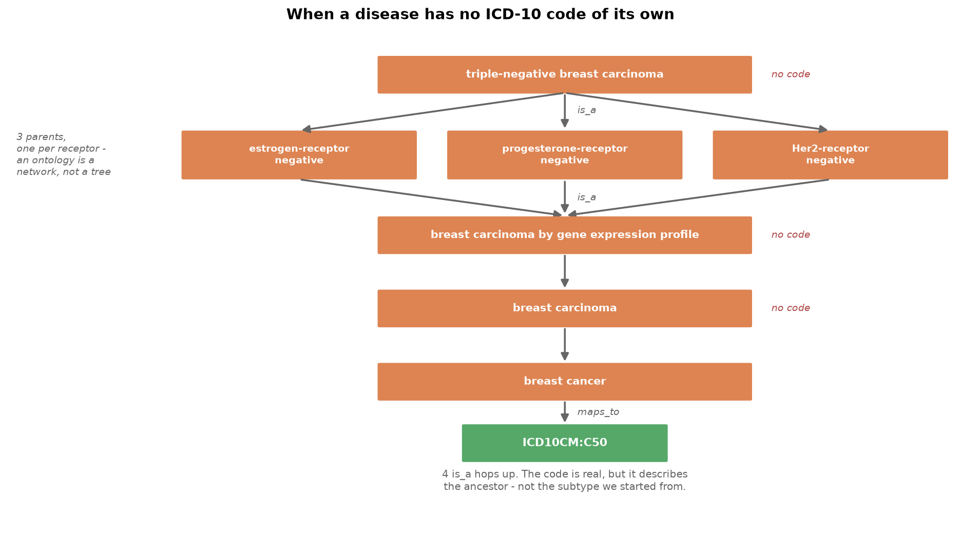
# Follow is_a edges upwards from triple-negative breast carcinoma. `with_depth`
# gives the number of hops, so we can tell "one level up" from "four levels up".
tnbc = "MONDO_0005494"

print(f"start: {G.nodes[tnbc]['name']}\n")
for ancestor, depth in h.ancestors_of(G, tnbc, with_depth=True):
    codes = [n for n in G.neighbors(ancestor) if G.nodes[n]["type"] == "icd10"]
    marker = f"   <-- {codes}" if codes else ""
    print(f"  {depth} hop(s) up: {G.nodes[ancestor]['name']}{marker}")
start: triple-negative breast carcinoma

  1 hop(s) up: progesterone-receptor negative breast cancer
  1 hop(s) up: Her2-receptor negative breast cancer
  1 hop(s) up: estrogen-receptor negative breast cancer
  2 hop(s) up: breast carcinoma by gene expression profile
  3 hop(s) up: breast carcinoma
  4 hop(s) up: breast cancer   <-- ['ICD10CM:C50']
Notice that three diseases sit one hop up: estrogen-receptor negative,
progesterone-receptor negative and Her2-receptor negative. That is not a quirk of
the data — it is the definition. “Triple-negative” means negative for all three
receptors, and the ontology records it as three separate is_a relationships.
So an ontology is a network, not a tree: a term can have several parents, and “climbing” means a breadth-first search rather than walking a single line. The helper sorts and searches by depth so the answer is the closest coded ancestor, and is identical every time we run it.
Mapping every disease#
h.icd10_for_disease(G, disease_id) wraps that climb. It returns the code, the
node it was found on, and how many hops it took — the steps field, where 0
means the disease carries the code itself.
Apply it to all 90 diseases and count how many can now be resolved.
'''
#################################################
                YOUR CODE HERE
#################################################

Climb the ontology for every disease and record what comes back.

`h.icd10_for_disease(G, d)` returns a dictionary. Call it once per disease and
store it, rather than calling it again for each key you need.

- Make an empty list called `rows`.
- Loop over `diseases`.
- For each disease `d`, call `h.icd10_for_disease(G, d)` and put the result in
  a variable called `result`.
- Append a dictionary to `rows` with three keys:
      "disease" -> the disease name,        `G.nodes[d]["name"]`
      "icd10"   -> the codes as one string, `", ".join(result["icd10"])`
      "steps"   -> how far we climbed,      `result["steps"]`
- Turn `rows` into a DataFrame called `resolved`.
'''

# --- SOLUTION ---
rows = []
for d in diseases:
    result = h.icd10_for_disease(G, d)

    rows.append({
        "disease": G.nodes[d]["name"],
        "icd10": ", ".join(result["icd10"]),
        "steps": result["steps"],
    })

resolved = pd.DataFrame(rows)
# --- END SOLUTION ---

n_resolved = resolved["icd10"].astype(bool).sum()
print(f"resolved: {n_resolved} / {len(diseases)}\n")
print(resolved["steps"].value_counts(dropna=False).sort_index().to_string())
resolved: 82 / 90

steps
0.0    19
1.0    10
2.0    19
3.0    21
4.0    12
5.0     1
NaN     8
From 19 to 82. Every breast cancer subtype now reaches C50, most of them 3–5 hops up.
But be careful what we claim. A code found 4 hops up is a real code, and it is what a hospital would have billed — but it describes the ancestor. Saying “triple-negative breast carcinoma maps to C50” is true; saying “C50 identifies triple-negative patients” is false. The mapping is many-to-one and it loses exactly the information a molecular study cares about.
# Which diseases still cannot be resolved?
resolved[~resolved["icd10"].astype(bool)]
| disease | icd10 | steps | |
|---|---|---|---|
| 30 | gastric carcinoma | NaN | |
| 38 | coronary artery disorder | NaN | |
| 43 | lung adenocarcinoma | NaN | |
| 48 | melanoma | NaN | |
| 52 | pancreatic ductal adenocarcinoma | NaN | |
| 57 | colorectal cancer | NaN | |
| 80 | rheumatoid arthritis | NaN | |
| 82 | glioblastoma | NaN |
These eight are genuine dead ends, and for a different reason from the subtypes.
Colorectal cancer, melanoma, glioblastoma, rheumatoid arthritis — every one of
these has a perfectly good ICD-10 code in the real world (C18, C43, C71,
M05). They are missing here because MONDO never curated the cross-reference, and
because these terms sit at the top of their own hierarchies so there is no ancestor
to inherit from either.
That is failure mode 2 from Part 2 — a plain curation gap, not a granularity mismatch. Two different causes, two different remedies, and the graph reports both as the same silence.
Section B — Which diseases share genes?#
ICD-10 got us in the door. Now the question the graph is genuinely good at.
Bipartite projection#
Our graph is close to bipartite: genes connect to diseases, and diseases to genes, but genes almost never connect to genes. (That is why the clustering coefficient in Part 2 was near zero.)
To ask “how similar are two diseases?”, we project the bipartite graph down onto the diseases alone — joining two diseases whenever they share genes.
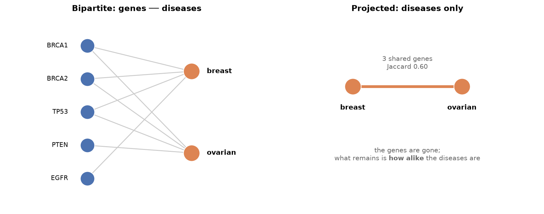
Similarity is measured with the Jaccard index: the size of the intersection over the size of the union. Using the raw count instead would just rank well-studied diseases highest, since they share genes with everything.
Comparing breast and ovarian cancer#
Find the genes shared by breast cancer (MONDO_0007254) and ovarian cancer
(MONDO_0008170), and compute the Jaccard index by hand before using the helper.
breast, ovarian = "MONDO_0007254", "MONDO_0008170"


# --- WORKED EXAMPLE - read this one, do not write it -------------------------
# Two gene sets, then the intersection. The very next exercise is these same
# three lines on a different graph, so read them now and you will be able to
# write them in a moment.
genes_breast = h.genes_for_disease(G, breast)
genes_ovarian = h.genes_for_disease(G, ovarian)

shared = genes_breast & genes_ovarian
jaccard = len(shared) / len(genes_breast | genes_ovarian)

print(f"breast:  {len(genes_breast)} genes")
print(f"ovarian: {len(genes_ovarian)} genes")
print(f"shared:  {len(shared)} genes,  Jaccard = {jaccard:.2f}\n")
print(sorted(G.nodes[g]["name"] for g in shared))
breast:  30 genes
ovarian: 30 genes
shared:  11 genes,  Jaccard = 0.22

['BRCA1', 'BRCA2', 'BRIP1', 'PIK3CA', 'TOP1', 'TOP2A', 'TP53', 'TUBA1B', 'TUBA1C', 'TUBB', 'TUBB3']
BRCA1, BRCA2, BRIP1 at the top of that list is a real result, and we derived it from graph structure alone.
Those three genes are the core of hereditary breast and ovarian cancer syndrome (HBOC) — the reason breast and ovarian cancer are screened for together, and the reason a BRCA1 carrier is counselled about both. We did not tell the graph that these two diseases were related. We asked which genes they had in common, and the syndrome fell out.
A caveat about that 0.22. Both diseases have exactly 30 genes here, because both hit the
--top-genes 30cap in the build script. Breast cancer’s weakest kept gene scores 0.61 and ovarian’s scores 0.53, against a stated cutoff of 0.05 — so everything between 0.05 and those values was discarded before we ever saw it.That means the union is pinned at 49 by construction, and the Jaccard index is measuring overlap between two top-30 lists, not overlap between two gene sets. The identity of the shared genes is trustworthy; the number is a property of the build script. Exactly the question this notebook keeps asking: did the data say that, or did the construction?
Exercise: Separate cause from treatment#
h.filter_by_datatype(G, evidence, datatypes) keeps only the associated_with
edges supported by particular kinds of evidence. h.CAUSAL_DATATYPES is
("genetic_association", "somatic_mutation") — the two that assert the gene has
something to do with causing the disease.
Build a causal-only graph and recompute the breast/ovarian overlap.
'''
#################################################
                YOUR CODE HERE
#################################################

Now do exactly the same thing again, but on a graph that keeps only causal
evidence. The three lines mirror the exercise above one for one.

- `h.filter_by_datatype(G, evidence, h.CAUSAL_DATATYPES)` returns a NEW graph
  containing only edges backed by genetic or somatic evidence. Call it `causal`.
- Get the two gene sets from `causal` exactly as before, with
  `h.genes_for_disease(causal, ...)`. Call them `causal_breast` and
  `causal_ovarian`.
- Intersect them with `&` and call the result `shared_causal`.
'''

# --- SOLUTION ---
causal = h.filter_by_datatype(G, evidence, h.CAUSAL_DATATYPES)

causal_breast = h.genes_for_disease(causal, breast)
causal_ovarian = h.genes_for_disease(causal, ovarian)

shared_causal = causal_breast & causal_ovarian
# --- END SOLUTION ---

print("all evidence:   ", sorted(G.nodes[g]["name"] for g in shared))
print("causal only:    ", sorted(G.nodes[g]["name"] for g in shared_causal))
print()
drug_only = h.filter_by_datatype(G, evidence, "known_drug")
print("known_drug only:", sorted(
    G.nodes[g]["name"] for g in
    h.genes_for_disease(drug_only, breast) & h.genes_for_disease(drug_only, ovarian)))
all evidence:    ['BRCA1', 'BRCA2', 'BRIP1', 'PIK3CA', 'TOP1', 'TOP2A', 'TP53', 'TUBA1B', 'TUBA1C', 'TUBB', 'TUBB3']
causal only:     ['BRCA1', 'BRCA2', 'BRIP1', 'PIK3CA', 'TP53']

known_drug only: ['PIK3CA', 'TOP1', 'TOP2A', 'TP53', 'TUBA1B', 'TUBA1C', 'TUBB', 'TUBB3']
Every tubulin disappears. What survives is BRCA1, BRCA2, BRIP1, PIK3CA
and TP53 — the actual hereditary breast-ovarian cancer genes. And the
known_drug list is now pure chemotherapy targets: tubulins and topoisomerases.
Note that PIK3CA and TP53 appear in both lists. That is not an error —
they are genuinely causal and genuinely drug targets. The evidence split does not
sort genes into clean bins; it tells us which claim we are relying on.
This is the answer to a question we should ask of every knowledge graph edge: what kind of statement is this, and is it the kind we need?
Getting the whole picture: Can we recover disease groups?#
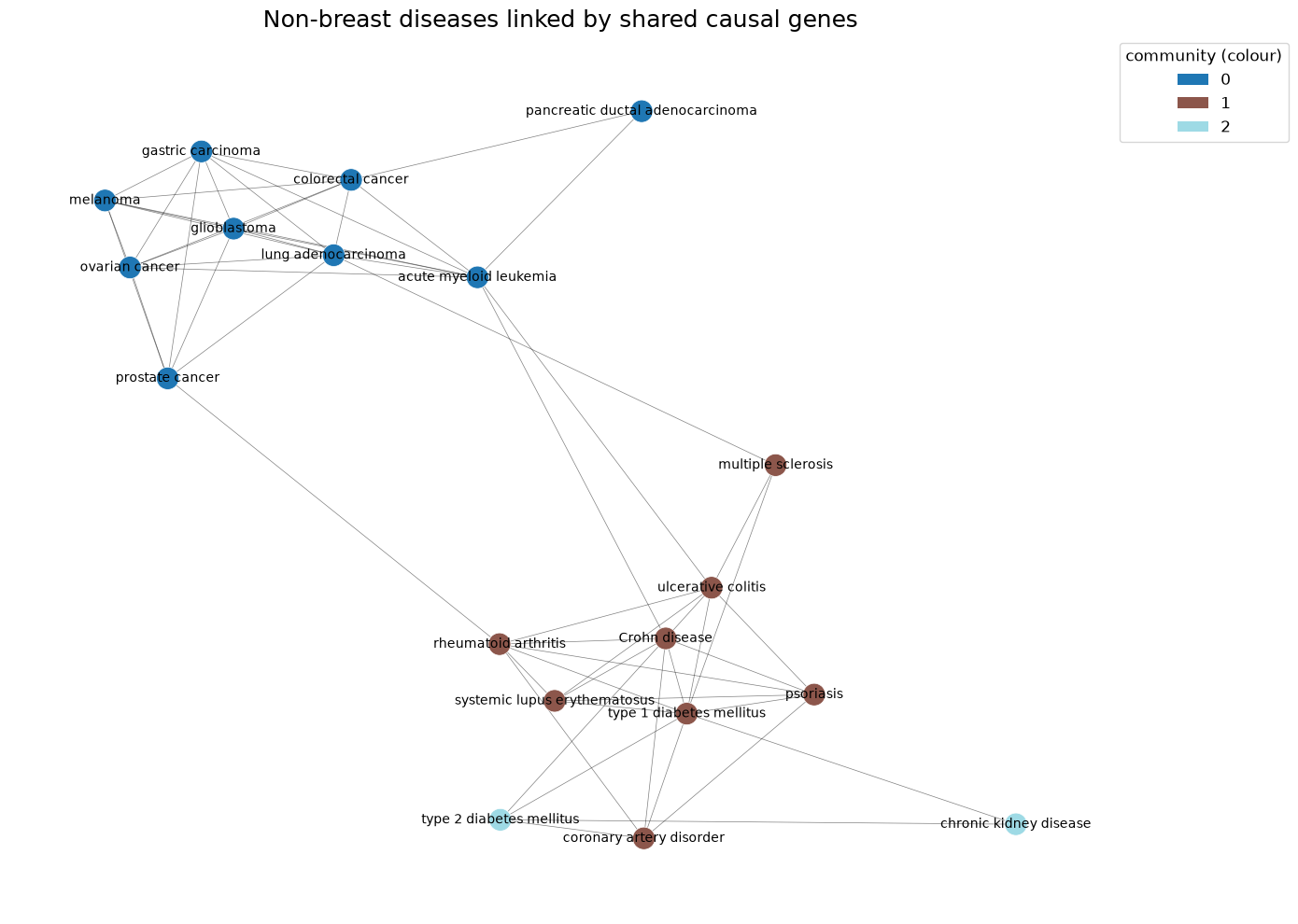
Now the payoff. Project all the non-breast diseases onto each other using causal evidence only, and run community detection — which knows nothing about cancer, autoimmunity or the clinic. It only sees which diseases share genes.
non_breast = [d for d in diseases if not is_breast(d)]
causal_projection = h.shared_gene_projection(causal, non_breast)

# Drop the weakest similarities so the communities are not linked by one gene.
strong = nx.Graph(
    (u, v, d) for u, v, d in causal_projection.edges(data=True) if d["weight"] >= 0.05
)
communities = nx.community.louvain_communities(strong, seed=0)

print(f"{len(non_breast)} diseases, {causal_projection.number_of_edges()} shared-gene "
      f"edges, {len(communities)} communities\n")
for i, community in enumerate(sorted(communities, key=len, reverse=True), start=1):
    print(f"Community {i}:")
    for name in sorted(G.nodes[d]["name"] for d in community):
        print(f"    {name}")
27 diseases, 69 shared-gene edges, 3 communities

Community 1:
    acute myeloid leukemia
    colorectal cancer
    gastric carcinoma
    glioblastoma
    lung adenocarcinoma
    melanoma
    ovarian cancer
    pancreatic ductal adenocarcinoma
    prostate cancer
Community 2:
    Crohn disease
    coronary artery disorder
    multiple sclerosis
    psoriasis
    rheumatoid arthritis
    systemic lupus erythematosus
    type 1 diabetes mellitus
    ulcerative colitis
Community 3:
    chronic kidney disease
    type 2 diabetes mellitus
# Draw it, colouring each disease by the community it landed in. Node labels are
# the disease names, so the grouping can be read off the picture directly.
labelled = nx.relabel_nodes(
    causal_projection.subgraph(strong.nodes()).copy(),
    {d: G.nodes[d]["name"] for d in strong.nodes()},
)
named_communities = [
    [G.nodes[d]["name"] for d in community] for community in communities
]

h.draw_network_with_node_attrs(
    labelled,
    communities=named_communities,
    title="Non-breast diseases linked by shared causal genes",
    figsize=(14, 10),
    node_size=300,
    with_labels=True,
)
What just happened (click to expand)
Nobody told the algorithm that cancers are cancers. It was given a set of diseases and, for each pair, the fraction of causal genes they share. Out came:
a cancer community — AML, colorectal, gastric, glioblastoma, lung adenocarcinoma, melanoma, ovarian, pancreatic, prostate
an autoimmune/inflammatory community — Crohn disease, ulcerative colitis, multiple sclerosis, psoriasis, rheumatoid arthritis, SLE, type 1 diabetes
a small metabolic/renal community — type 2 diabetes and chronic kidney disease
That is the clinical taxonomy, recovered from gene sharing alone. It is the single best argument for representing biomedical knowledge as a graph: structure that nobody encoded turns out to be recoverable from the structure that somebody did.
Only 19 of the 27 diseases end up in a community, and the absentees are as informative as the members. Alzheimer disease, Parkinson disease and schizophrenia each have causal genes in the graph — 13, 7 and 11 of them — but share almost none with anything else here, so no edge clears the threshold. The brain diseases are genetically their own world. Asthma and osteoporosis are isolated for the same reason. Three more terms have no causal genes at all and so cannot be placed either way.
Not clustering is a result. It is not the same as being unstudied.
One result is worth arguing about. Coronary artery disorder lands with the autoimmune diseases rather than with the metabolic ones. Is that a mistake, or is it the graph noticing that atherosclerosis is an inflammatory disease? Both readings are defensible, and deciding between them needs a cardiologist, not more code.
Try re-running the cell above with h.filter_by_datatype(G, evidence, "known_drug")
instead of causal. The communities re-form around shared treatments rather than
shared biology, and diseases that have nothing in common mechanistically end up
adjacent. Same algorithm, same graph, different question.
Section C — Connecting to the omics data#
Stretch section. If the room is short of time, stop here and come back to this afterwards — it needs the Session 2 omics pickle, and Section B is the part that carries the practical. Nothing later depends on finishing it live.
This graph is not a closed world. It is keyed to join onto the molecular data from Session 2.
The identifier trap#
The TCGA transcriptomics matrix uses versioned Ensembl IDs — ENSG00000012048.23.
Open Targets uses unversioned ones — ENSG00000012048. The suffix is the
annotation release the gene model came from.
Join them naively and we match nothing at all. Not fewer things — nothing. And because an empty join is not an error, it looks like a real biological result.
# Set this to wherever the Session 2 omics pickle lives.
OMICS_PATH = "/data/omics.pkl"

try:
    layers, meta = h.load_omics(OMICS_PATH, layers=("transcriptomics",))
    transcriptomics = layers["transcriptomics"]
    OMICS_AVAILABLE = True
    print(f"transcriptomics: {transcriptomics.shape[0]} patients "
          f"x {transcriptomics.shape[1]:,} genes")
    print(f"subtype labels:  {meta.value_counts().to_dict()}")
except FileNotFoundError as exc:
    OMICS_AVAILABLE = False
    print(f"Skipping Section C - {exc}")
transcriptomics: 500 patients x 29,995 genes
subtype labels:  {'LumA': 237, 'LumB': 100, 'Basal': 97, 'Her2': 41, 'Normal': 25}
if OMICS_AVAILABLE:
    kg_genes = set(h.nodes_of_type(G, "gene"))
    omics_raw = set(transcriptomics.columns)
    omics_stripped = set(h.strip_ensembl_version(transcriptomics.columns))

    print(f"matched WITHOUT stripping the version: {len(kg_genes & omics_raw):>4}")
    print(f"matched AFTER stripping the version:   {len(kg_genes & omics_stripped):>4}"
          f"  ({len(kg_genes & omics_stripped) / len(kg_genes):.1%} of KG genes)")
matched WITHOUT stripping the version:    0
matched AFTER stripping the version:    737  (97.0% of KG genes)
Zero versus 737. One .split(".")[0] is the difference between a working analysis
and a silently empty one.
Why zero is the safe answer#
That zero is not a data quality problem. It is arithmetic: 100% of the TCGA columns carry a version suffix and none of the Open Targets ids do, so the two sets cannot overlap. We would get zero even if both datasets were flawless.
And zero is the failure we want, because nobody interprets an empty result as biology. We notice immediately and go and fix it.
The dangerous case is the near miss. Suppose the suffix were present on only some columns, and the join returned 12 genes out of 760. Nothing errors. The analysis runs, the figures render, the enrichment comes back with plausible terms — and we publish a conclusion drawn from 1.6% of the data while believing we used all of it. A partial join looks like a result. An empty one looks like a bug.
So the rule is not “check the join is non-empty”. It is:
Check the join is the size we expected. Predict the number before running it, and treat any disagreement as a bug until it has been explained.
Here we predicted ~760 and got 737. The gap is small enough to check by hand:
if OMICS_AVAILABLE:
    unmatched = kg_genes - omics_stripped
    print(f"{len(unmatched)} KG genes are not in the transcriptomics matrix:")
    for gene in sorted(G.nodes[g]["name"] for g in unmatched):
        print(f"   {gene}")
23 KG genes are not in the transcriptomics matrix:
   CASR
   CHRM2
   CTRB1
   CTRB2
   DRD3
   HTR3B
   HTR3C
   HTR3D
   HTR3E
   HTR5A
   IL17A
   IL17F
   INS
   MIF
   NEUROD1
   OPRM1
   PAX4
   PDE4C
   SLC2A2
   TNP1
   TREX1
   TYR
   ZAR1L
Read that list and the pattern is obvious. INS, PAX4, SLC2A2 and CTRB1/2
are pancreatic; HTR3B–HTR3E, HTR5A, DRD3, CHRM2 and OPRM1 are
neurotransmitter receptors; IL17A/F and MIF are immune; TYR is a melanocyte
gene; TNP1 is testis-specific and ZAR1L oocyte-specific.
Every one entered the graph through a comparison disease — diabetes, schizophrenia, Parkinson disease, the autoimmune group, melanoma — and none would be expressed in breast tissue. Their absence is the correct answer, which is what lets us accept 737 as the expected number rather than a warning sign.
One trap worth knowing about even though this matrix avoids it: TCGA gene tables
often carry pseudoautosomal genes as ENSG00000182378.14_PAR_Y. Those strip to
the same id as their X-chromosome counterpart, creating duplicate columns that
silently corrupt the join. Checking for duplicates after stripping costs one line
and this matrix has none.
The PAM50 subtypes are nodes in this graph#
Session 2 predicts a patient’s PAM50 subtype: LumA, LumB, Basal, Her2 or Normal.
Every one of those five labels is a disease node here. So a prediction from Session 2 is not just a string — it is an entry point into the knowledge graph.
if OMICS_AVAILABLE:
    subtype_table = pd.DataFrame([
        {
            "PAM50": label,
            "patients": int((meta == label).sum()),
            "MONDO id": mondo_id,
            "name in graph": G.nodes[mondo_id]["name"],
            "genes in graph": len(h.genes_for_disease(G, mondo_id)),
        }
        for label, mondo_id in h.PAM50_TO_MONDO.items()
    ])
    display(subtype_table)
| PAM50 | patients | MONDO id | name in graph | genes in graph | |
|---|---|---|---|---|---|
| 0 | LumA | 237 | MONDO_0021116 | luminal A breast carcinoma | 30 |
| 1 | LumB | 100 | MONDO_0021115 | luminal B breast carcinoma | 30 |
| 2 | Basal | 97 | MONDO_0004984 | basal-like breast carcinoma | 0 |
| 3 | Her2 | 41 | MONDO_0006244 | HER2 positive breast carcinoma | 30 |
| 4 | Normal | 25 | MONDO_0006324 | normal breast-like subtype of breast carcinoma | 19 |
Note Basal again: 97 patients in the omics data, 0 genes in the graph. The
molecular data has plenty to say about these patients; the knowledge graph does
not, because of the vocabulary mismatch from Part 2. Sending a Basal patient’s gene
list into this graph, we would need to reason about triple-negative breast carcinoma instead — which is precisely the kind of step an agent has to get right
in Session 4.
Exercise: from a gene list to a disease#
The smallest useful knowledge graph query, and the shape of every query in Sessions 3 and 4: given a set of genes, which diseases do they touch?
Take the most variable genes in the transcriptomics matrix and look them up.
if OMICS_AVAILABLE:

        # --- WORKED EXAMPLE ------------------------------------------------------
    # Rank the genes by variance and keep the top 200. Given rather than asked
    # because this section is optional and depends on the omics file.
    gene_variance = transcriptomics.var(axis=0)
    gene_variance = gene_variance.sort_values(ascending=False)
    variable_genes = gene_variance.head(200).index

    mapped = h.map_genes_to_kg(G, variable_genes)
    print(f"{mapped['in_kg'].sum()} of {len(mapped)} most-variable genes "
          f"are in the knowledge graph\n")
    display(mapped[mapped["in_kg"]].head(10))
10 of 200 most-variable genes are in the knowledge graph
| input_id | ensembl_id | in_kg | symbol | degree | |
|---|---|---|---|---|---|
| 21 | ENSG00000181092.10 | ENSG00000181092 | True | ADIPOQ | 1 |
| 34 | ENSG00000164756.12 | ENSG00000164756 | True | SLC30A8 | 1 |
| 48 | ENSG00000082175.15 | ENSG00000082175 | True | PGR | 1 |
| 50 | ENSG00000162896.6 | ENSG00000162896 | True | PIGR | 1 |
| 78 | ENSG00000091831.24 | ENSG00000091831 | True | ESR1 | 25 |
| 95 | ENSG00000181143.15 | ENSG00000181143 | True | MUC16 | 2 |
| 124 | ENSG00000156234.7 | ENSG00000156234 | True | CXCL13 | 1 |
| 126 | ENSG00000129514.8 | ENSG00000129514 | True | FOXA1 | 6 |
| 130 | ENSG00000179023.8 | ENSG00000179023 | True | KLHDC7A | 1 |
| 191 | ENSG00000178568.15 | ENSG00000178568 | True | ERBB4 | 6 |
if OMICS_AVAILABLE:
    display(h.diseases_for_genes(G, variable_genes, top_n=10))
| disease_id | name | n_genes | mean_score | genes | |
|---|---|---|---|---|---|
| 0 | MONDO_0021115 | luminal B breast carcinoma | 3 | 0.331667 | ERBB4, ESR1, FOXA1 |
| 1 | MONDO_0003024 | breast angiosarcoma | 2 | 0.074850 | ADIPOQ, PIGR |
| 2 | MONDO_0004988 | breast adenocarcinoma | 2 | 0.539550 | ESR1, FOXA1 |
| 3 | MONDO_0005298 | osteoporosis | 2 | 0.577850 | ESR1, PGR |
| 4 | MONDO_0000552 | breast lobular carcinoma | 2 | 0.379500 | ESR1, FOXA1 |
| 5 | MONDO_0004950 | gastric carcinoma | 2 | 0.382250 | ERBB4, ESR1 |
| 6 | MONDO_0006116 | breast carcinoma by gene expression profile | 2 | 0.370000 | ESR1, FOXA1 |
| 7 | MONDO_0005590 | breast ductal adenocarcinoma | 2 | 0.383350 | ESR1, FOXA1 |
| 8 | MONDO_0005063 | medullary breast carcinoma | 2 | 0.139350 | ESR1, MUC16 |
| 9 | MONDO_0003624 | acinic cell breast carcinoma | 2 | 0.231250 | ERBB4, ESR1 |
Whatever comes back, apply the scepticism from Section B before believing it. Ask:
Are these diseases hit by specific genes, or by promiscuous ones like
TP53?Are the breast subtypes at the top because the biology says so, or because 63 of this graph’s 90 diseases are breast cancer subtypes?
ESR1andFOXA1drive most of these hits. Is that a finding, or is it just that the most variable genes in a breast tumour matrix are the hormone-receptor genes, which are also the best-annotated breast cancer genes in Open Targets?
The circularity is real and worth stating. Notice, though, that
osteoporosis and gastric carcinoma also appear — diseases that share ESR1
for genuinely different reasons. Working out which hits are informative and which
are structural is the whole skill.
Section D — Combining networks#
Closing section. Unlike Section C this needs no external file: the expression matrix is committed in
/data/session-1-data/. If time is short, read the results rather than running them.
Part 1 built two networks over the same 737 genes — an computed co-expression network computed from measurements, and this curated knowledge graph read from recorded facts. Section B then taught us to filter curated edges by the kind of evidence behind them.
Put those together and we get the question the whole tutorial is named after: can molecular data strengthen the evidence for a gene–disease relationship?
The recipe is three lines. Take the genes with causal evidence for breast cancer — our best curated answer. Ask which genes co-express with them. Then sort what comes back by what the graph already says about it.
Co-expression says |
Knowledge graph says |
Reading |
|---|---|---|
correlated |
causal edge already |
corroboration — two independent routes |
correlated |
non-causal edge only |
evidence upgrade, or a shared confound |
correlated |
no edge to this disease |
candidate |
expression = h.load_expression()
correlations = h.correlation_matrix(expression)

# The curated answer: genes with genetic or somatic evidence for breast cancer.
causal_graph = h.filter_by_datatype(G, evidence, h.CAUSAL_DATATYPES)
causal_genes = h.genes_for_disease(causal_graph, breast)
all_breast_genes = h.genes_for_disease(G, breast)

seeds = sorted(causal_genes & set(correlations.index))
print(f"breast cancer: {len(all_breast_genes)} genes, "
      f"{len(causal_genes)} of them causal, {len(seeds)} of those measured")
print(sorted(G.nodes[g]["name"] for g in seeds))
breast cancer: 30 genes, 16 of them causal, 16 of those measured
['ATM', 'BARD1', 'BRCA1', 'BRCA2', 'BRIP1', 'CCND1', 'CHEK2', 'EGFR', 'ESR1', 'FGFR2', 'NBN', 'PALB2', 'PIK3CA', 'PRIM1', 'TP53', 'VEGFA']
Do the causal genes corroborate each other?#
Before looking for anything new, a sanity check. If co-expression carries real signal about breast cancer biology, the genes we already believe cause breast cancer should show some of it among themselves.
import itertools

pairs = pd.DataFrame([
    {"gene_a": G.nodes[a]["name"], "gene_b": G.nodes[b]["name"],
     "r": round(correlations.at[a, b], 3)}
    for a, b in itertools.combinations(seeds, 2)
])
strong = pairs[pairs["r"].abs() >= 0.5].sort_values("r", key=abs, ascending=False)

print(f"{len(strong)} of {len(pairs)} causal gene pairs co-express at |r| >= 0.5")
display(strong.head(6))
10 of 120 causal gene pairs co-express at |r| >= 0.5
| gene_a | gene_b | r | |
|---|---|---|---|
| 93 | BRIP1 | BRCA2 | 0.659 |
| 92 | BRIP1 | BARD1 | 0.658 |
| 99 | BARD1 | BRCA2 | 0.600 |
| 98 | BRIP1 | PRIM1 | 0.581 |
| 43 | ESR1 | CCND1 | 0.571 |
| 14 | BRCA1 | PRIM1 | 0.569 |
Ten of 120 pairs — and look at which ten. BRCA2–BRIP1, BARD1–BRIP1,
BARD1–BRCA2: the homologous-recombination repair complex, recovered from
expression alone. The graph knows these genes cause breast cancer because families
were sequenced. The expression matrix knows they belong together because they are
transcribed together. Two entirely independent routes to the same biology —
that is what corroboration looks like, and it is the strongest evidence pattern
available to us.
Note also that 110 of 120 pairs show nothing. TP53 and ESR1 both cause
breast cancer and have no reason to co-express. Corroboration is a bonus when it
appears, never a requirement.
What else tracks the causal genes?#
Now outwards. Which genes co-express with the causal set, and what does the graph already say about them?
# --- WORKED EXAMPLE - read this one, do not write it -------------------------
# The same list-of-dictionaries shape once more, with a three-way if/elif/else
# deciding what the graph already says about each gene. Given rather than asked
# so the session can end on the result instead of on the typing.
rows = []
for gene in correlations.index:
    if gene in seeds:
        continue

    n_partners = int((correlations.loc[gene, seeds].abs() >= 0.5).sum())
    if n_partners == 0:
        continue

    if gene in causal_genes:
        kg_link = "causal"
    elif gene in all_breast_genes:
        kg_link = "non-causal"
    else:
        kg_link = "none"

    rows.append({
        "symbol": G.nodes[gene]["name"],
        "n_causal_partners": n_partners,
        "kg_link": kg_link,
    })

candidates = pd.DataFrame(rows)
candidates = candidates.sort_values(["n_causal_partners", "symbol"],
                                    ascending=[False, True])

print(candidates["kg_link"].value_counts().to_string())
print("\nnon-causal breast cancer edges among them:",
      sorted(candidates.loc[candidates["kg_link"] == "non-causal", "symbol"]))
display(candidates.head(15))
kg_link
none          184
non-causal      7

non-causal breast cancer edges among them: ['CDK6', 'TOP1', 'TOP2A', 'TUBA1B', 'TUBA1C', 'TUBB', 'TYMS']
| symbol | n_causal_partners | kg_link | |
|---|---|---|---|
| 116 | BUB1B | 6 | none |
| 14 | HMMR | 6 | none |
| 73 | TOP2A | 6 | non-causal |
| 177 | BLM | 5 | none |
| 146 | EXO1 | 5 | none |
| 100 | FANCD2 | 5 | none |
| 91 | KNL1 | 5 | none |
| 29 | POLA1 | 5 | none |
| 150 | TYMS | 5 | non-causal |
| 65 | MCM8 | 4 | none |
| 57 | MSH6 | 4 | none |
| 28 | POLE2 | 4 | none |
| 70 | PPAT | 4 | none |
| 104 | PRIM2 | 4 | none |
| 10 | RAD51 | 4 | none |
Read the kg_link column before the gene names.
Seven genes carry a non-causal breast cancer edge: TOP2A, TYMS, TUBA1B,
TUBA1C, TUBB, TOP1, CDK6. These are precisely the genes Section B4 worked
to remove — the chemotherapy targets that entered through known_drug evidence.
Co-expression has handed them straight back.
That is worth sitting with. We filtered them out because their curated edge was a
statement about treatment. They return because they are proliferation genes, and
in a tumour cohort everything proliferative correlates with everything else
proliferative — the same confound Part 1 found around BRCA1. Two different
methods, two different reasons, the same wrong genes. Agreement between two
sources is only evidence if their errors are independent, and here they are not.
The remaining 184 have no breast cancer edge at all — the candidate column. And the top of that list is genuinely mixed:
BLM,EXO1,FANCD2,RAD51,MSH6,MCM8— DNA repair and genome stability genes. Several are real hereditary cancer genes in the wider literature; our graph simply has no breast cancer edge for them. These are candidates worth taking seriously.BUB1B,HMMR,KNL1,POLA1,POLE2,PRIM2,RRM2— mitosis and replication. The proliferation confound again, now with no curated edge to warn us about it.
The two groups are interleaved in the ranking, and no column in this table
separates them. BUB1B and HMMR sit at the very top with six causal partners
each; RAD51 sits below them with four. Nothing in the data says which is which —
that judgement takes biological knowledge about why two genes might correlate.
That is the honest state of the method, and it is the right place to stop:
The knowledge graph alone gives us what is already known, with its silences.
The expression data alone gives us correlations, with a dominant confound.
Together they give us a ranked, interpretable shortlist — and a new failure mode created by the combination itself.
Where this goes next. Sessions 3 and 4 hand this exact problem to an LLM agent: plan the traversal, pull the evidence, and judge which candidates survive. The gaps from Section A, the treatment-versus-cause distinction from Section B, and the interleaved list above are what such an agent has to get right — and are how we will check whether it did.
Summary#
Section A — ICD-10
ICD-10 is the clinical vocabulary, subdivided anatomically, not molecularly.
Coverage is not evenly distributed: 3 of 63 breast subtypes carry a code against 16 of 27 other diseases. The failure is specific to fine granularity.
Climbing
is_araises coverage from 19 to 82 of 90 — but an inherited code describes the ancestor, and the mapping is many-to-one.The eight remaining failures are a different problem: plain curation gaps for diseases that do have codes in the real world. The graph reports both silences identically.
Section B — shared genes
Projecting the bipartite graph onto diseases turns “which diseases resemble each other?” into a structural question.
Breast × ovarian recovers BRCA1/BRCA2/BRIP1 — HBOC, from graph structure alone.
It also surfaces tubulins and topoisomerases, shared because of chemotherapy rather than biology. The overall association score cannot tell the two apart.
Filtering to
genetic_associationandsomatic_mutationcan: every tubulin disappears and the real hereditary genes remain. Always ask what kind of claim an edge is making.Community detection on causal evidence alone recovers the clinical taxonomy — cancers, autoimmune diseases, metabolic diseases — without being told any of it.
Section C — omics (stretch)
Versioned vs unversioned Ensembl IDs: 0 matches vs 737. Predict the join size before running it; an empty join is safe, a partial one is dangerous.
All five PAM50 subtypes are disease nodes, so a Session 2 prediction is a graph entry point.
Section D — both networks together
The causal breast cancer genes partly corroborate each other in expression (
BRCA2/BRIP1/BARD1, the HR complex) — two independent routes, one biology.Co-expression re-introduces the exact chemotherapy targets Section B removed. Two sources agreeing is only evidence when their errors are independent.
184 genes co-express with the causal set and have no curated breast cancer edge. Real repair-gene candidates and proliferation artefacts are interleaved, and no column in the table tells them apart.
Where this goes next: Session 3 builds LLM agents that plan these traversals, and Session 4 has us query the graph from a multi-omics profile. Everything above — the gaps, the inherited codes, the technically-correct-but-misleading edges — is what those agents have to get right, and what we need to check them against.